Objective
We show how to estimate the Markov chain transition matrix and initial probability distribution vector that fit a sequence of observations.
Example
Example 1: Suppose 10 runs of a Markov process of length 20 (labelled A-J) result in the output shown in Figure 1. Find the most likely transition matrix and distribution vector.
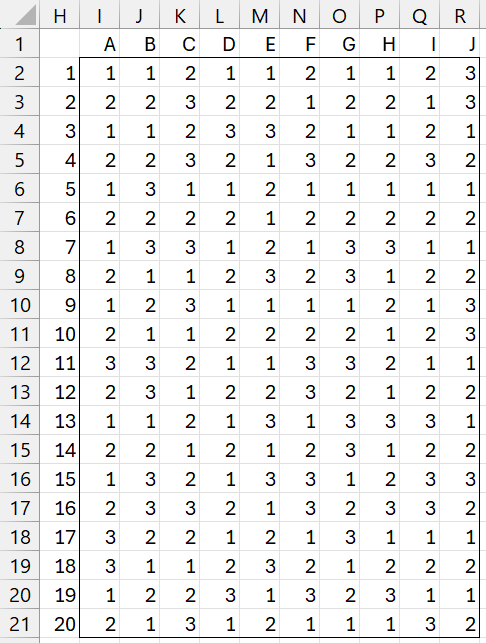
Figure 1 – Observed states
In general, if there are m runs, each of length n, and states 1, …, k, where nij is the number of transitions from state i to state j, then we can estimate the transition probability pij by
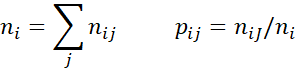
If ni = 0, then the data doesn’t help us estimate pij, and so we can simply use the following estimate:
pij = 1/k
It turns out that these estimates are the best estimates available, i.e. they produce the least error.
Results
For Example 1, we estimate the pij as shown in Figure 2.
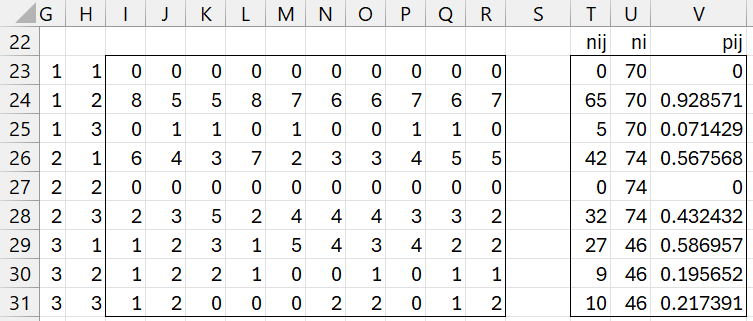
Figure 2 – Estimating the transition probabilities
Each row in the figure calculates one of the 3 × 3 = 9 transition probabilities. E.g. row 24 calculates the transition probability p12 (the values shown in columns G and H). The values in columns I through R show the nij values for each of the 10 runs. E.g. for the first run, n12 = 8, as shown in cell I24. These values are calculated by placing the formula
=SUM(IF(I$2:I$20=$G23,IF(I$3:I$21=$H23,1,0),0))
in cell I23, highlighting range I23:R31, and pressing Ctrl-R and Ctrl-D. The total nij values are simply the sum of the nij values for each of the 10 runs. These are shown in range T23:T31, and are calculated by placing the formula =SUM(I23:R23) in cell T23, highlighting range T23:T31, and pressing Ctrl-D.
Now, n1 = 0 + 65 + 5 = 70, as shown in cell U23, and repeated in cells U24 and U25. We calculate n2 and n3 similarly. We obtain the nine pij values by placing the formula T23/U23 in cell V23, highlighting range V23:V31, and pressing Ctrl-D. After transferring these values into the transition matrix, we obtain the output shown in range Y24:AA26 of Figure 3.
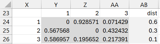
Figure 3 – Transition matrix and initial distribution vector
We can also estimate the initial distribution vector, as shown in column AB of Figure 3, by placing the formula =COUNTIF(I$2:R$2,X24)/COUNT(I$2:R$2) in cell AB24, highlighting range AB24:AB26, and pressing Ctrl-D. Note that these values are obtained using only the first row of the data from Figure 1.
Worksheet Function
The Real Statistics Resource Pack provides the following function to simplify the process of obtaining this estimate from the observed state data in R1.
MarkovParams(R1, k): returns a k × k+1 array, where the leftmost k × k array is the estimated transition matrix and the rightmost k × 1 column array is the estimated distribution.
Here, k defaults to the largest element in R1.
Actually, this function handles the situation where the runs are not of equal length. In this case, the number of rows in R1 equals the size of the longest run. Runs of smaller length correspond to columns with terminating zero or blank entries (zero functions as a blank).
Thus, the output in range Y24:AB26 can be obtained using the array formula
=MarkovParams(I2:R21)
Observation
The observations in Figure 1 were created using the MarkovSim function from the Markov model described in Example 3 of Markov Chain Real Statistics Support. Note that the values in the transition matrix shown in Figure 3 are pretty close to those shown in Figure 4 of Markov Chain Real Statistics Support.
Links
Examples Workbook
Click here to download the Excel workbook with the examples described on this webpage.
Reference
Stack Exchange (2023) Estimating Markov chain transition probabilities from data
https://stats.stackexchange.com/questions/605077/estimating-markov-chain-transition-probabilities-from-data
Bouman, C. A. (2006) Markov chains and Hidden Markov models
https://engineering.purdue.edu/~bouman/ece641/previous/fall06/notes/pdf/MC-HMMs.pdf
Leskela, L., Dreveton, M. (2026) Robust estimation of a Markov chain transition matrix from multiple samplepaths
https://onlinelibrary.wiley.com/doi/full/10.1111/stan.70023