On this web page, we describe some of the support that the Real Statistics Resource Pack provides for Markov chains.
Data Analysis Tool
Starting with Rel 9.9, the Real Statistics Resource Pack provides a way to draw a transition diagram for a Markov chain.
Example 1: Draw the diagram for the Markov chain with the transition matrix shown in range B2:E5 of Figure 1.
Before using the data analysis tool, you also need to create a node range as shown in range B8:C11 of Figure 1. The values in the node range are the (x, y) coordinates of the nodes in the network diagram (corresponding to the 4 states in the chain).
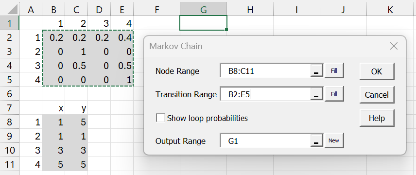
Figure 1 – Markov Chain Diagram dialog box
Press Ctrl-m, and select Markov Chain Diagram from the Corr tab. Fill in the dialog box that appears as shown on the right side of Figure 1. The output appears in Figure 2.
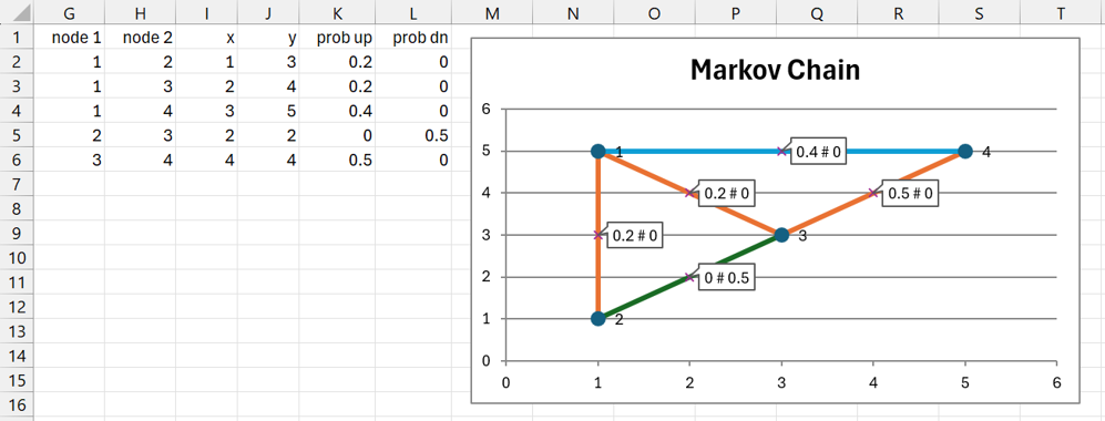
Figure 2 – Transition Diagram
Output description
The table on the left of Figure 2 describes the edges of the diagram. E.g. the midpoint of the edge between nodes 1 and 2 has coordinates (1, 3) (cells I2 and J2). The probability p12 = .2 (cell K2), lower node # to higher node #, and p21 = 0 (cell L2), higher node # to lower node #. This is shown in the diagram as .2 # 0 at the coordinates (1, 3).
The diagram on the right shows the same sort of information. Note that three edges start from node 1. These represent the probabilities .2 to node 2, .2 to node 3, and .4 to node 4. This leaves 1 – (.2+.2+.4) = .2, which represents p11, not shown in the diagram.
If you want to see the loop probabilities on the diagram, then you need to check the Show loop probabilities option in Figure 1. In this case, the transition diagram is shown in Figure 3.
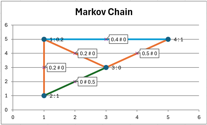
Figure 3 – Show loop probabilities
You see that the label for node 1 is 1 : .02, which means that p11 = .02.
Worksheet Functions
Starting with Rel 9.9, the Real Statistics Resource Pack provides the following worksheet function. Here, Rp is the k × k transition matrix P for states S = {1, 2, …, k}, and Rd is the k × 1 initial distribution array π.
MarkovProb (Rp, Rd, n): returns a k × 1 distribution array for xn, i.e. πPn
The second argument can also take an integer value j, from 1 to k. In this case, Rd is assumed to be a column array all of whose values are zero except for 1 in the jth position.
The Real Statistics Resource Pack will also provide several worksheet functions for the simulation of a Markov chain.
MarkovSim(Rp, Rd, n): returns a column array with n entries from the simulation of a Markov chain based on the k × k transition matrix in Rp and k × 1 initial distribution array Rd. As for MarkovProb, the second argument can take an integer value between 1 and k.
MarkovSimProb(Rp, Rd, n, m): returns a k × 1 distribution array with an estimated xn based on the average of the distribution values from m simulations.
Examples
Example 2: For the Markov chain of Example 1, we obtain the output for , as shown in Figure 4. Here, range H2:H5 contains the formula =MarkovProb(B2:E5,G2:G5,20) and K2:K5 contains the formula =MarkovProb(B2:E5,J2:J5,20). We can also obtain this second result by using the formula =MarkovProb(B2:E5,3,20).
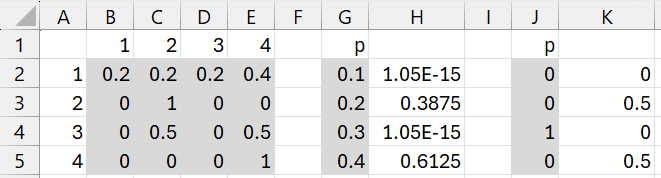
Figure 4 – MarkovProb function
Example 3: Create a simulation of a Markov chain of length 20 based on the transition matrix in range B2:D4 of Figure 5 and the initial distribution shown in range F2:F4.
The result is shown in range I1:I20 using the formula =MarkovSim(B2:D4, F2:F4, 20).
We obtain the simulation shown in range J1:J20 based on the initial distribution shown in range G2:G4 using either formula =MarkovSim(B2:D4, G2:G4, 20) or =MarkovSim(B2:D4, 3,20).
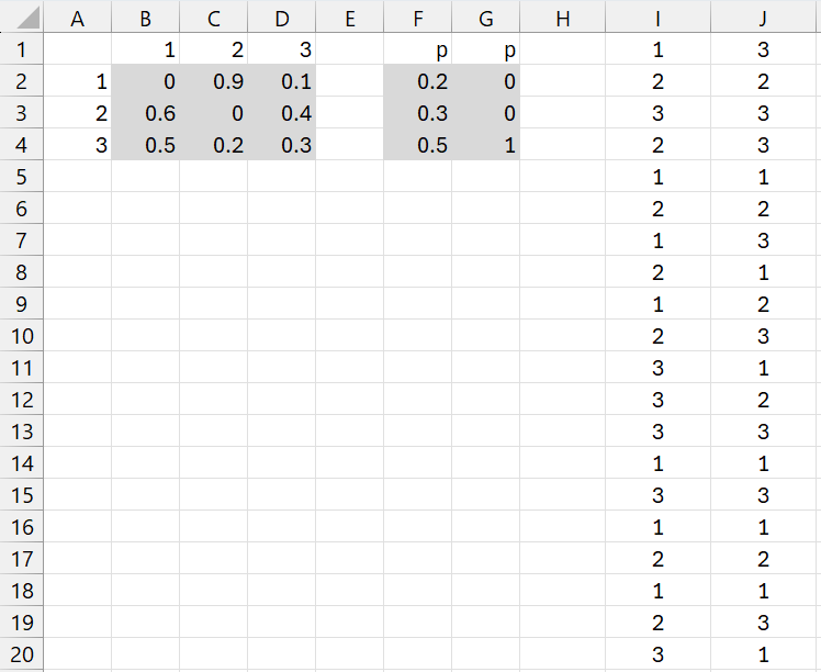
Figure 4 – MarkovSim function
Example 4: For the Markov chain and initial distribution of Example 3, find πPn. See how this value compares with the value obtained via 100 simulations.
The result is shown in range H2:H4 of Figure 5 using the formula =MarkovProb(B2:D4, F2:F4, 20).
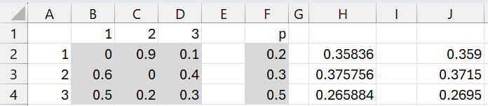
Figure 5 – MarkovSimProb function
The output from the simulation is shown in range J2:J4 using the formula =MarkovSimProb(B2:D4, F2:F4, 20, 100).
Other worksheet functions
Additional worksheet functions are described at
Examples Workbook
Click here to download the Excel workbook with the examples described on this webpage.
Links
References
Aldridge, M. (2021) Hitting times. Introduction to Markov Processes
https://mpaldridge.github.io/math2750/S08-hitting-times.html
Norris, J. (2004) Discrete-time Markov chains. Cambridge University Press
https://www.statslab.cam.ac.uk/~jrn10//Markov/
Sargent, T. J., Stachurski, J. (2025) Markov chains: Basic concepts. First course in quantitative economics with Python
https://intro.quantecon.org/markov_chains_I.html
Tolver, A. (2016) Introduction to Markov chains
https://www.math.ku.dk/bibliotek/arkivet/noter/stoknoter.pdf