Gambler’s Ruin

On this web page, we describe the gambler’s ruin Markov chain. This allows us to demonstrate many of the concepts from Hitting Probabilities.

Description

Player A starts with $a and player B starts with $b. On each turn, they bet $1. The probability that A wins is p and the probability that B wins is q, with p + q = 1. The game continues until one player runs out of money. What is the probability that A goes broke, and what is the probability that B goes broke?

Let m = a + b. We use the sample space S = {0, 1, …, m}. Here, x_n = the amount of money held by A, where x₀ = a and the transition probabilities are

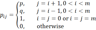
The probability that A goes broke given that he starts with $i is h_i0.

h_i0 = P(x_n = 0 for some n | x₀ = a)

But

h_i0 = ph_i+1,0 + qh_i-1,0          h₀₀ = 1     h_m0 = 0

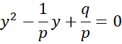
This is a homogeneous difference equation of form

Hitting probabilities

Property 1: The probability that Player A will go broke in the gambler’s ruin game is

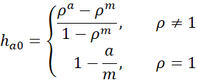
where ρ = q/p.

Proof: The characteristic equation is

The roots of this equation are

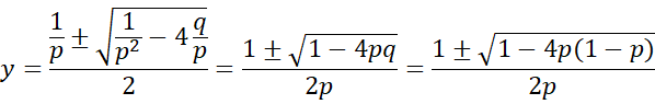
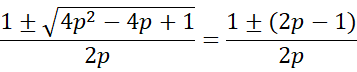
Thus, the roots are 1 and ρ = (1–p)/p = q/p

One root case

Suppose p = ½, then q = ½, and so there is one distinct root 1/(2p) = 1. The solution, therefore, takes the form

h_i0 = A + Bi)1ⁱ = A + Bi

Using the initial conditions, we see that

1 = h₀₀ = A + B(0) = A

0 = h_m0 = A + B(m) = 1 + Bm

Thus, B = –1/m and A = 1. Therefore, the solution takes the form

h_i0 = A + Bi = 1 – i/m

Two distinct real roots case

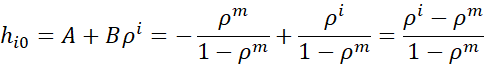
Since the roots are 1 and ρ, the solution takes the form

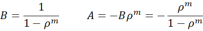
Using the initial conditions, we see that

1 = h₀₀ = A + Bρ⁰ = A + B

0 = h_m0 = A + Bρ^m

Hence

A = –Bρ^m

1 = A + B = –Bρ^m + B = (1–ρ^m)B

It now follows that

Limiting case

In the case where Player B has a huge cash reserve (e.g. Player B is a casino), we can estimate h_a0 by using the limit when b → ∞ (or equivalently when m → ∞). Also, suppose that the odds are in favor of Player B (i.e. q > p).

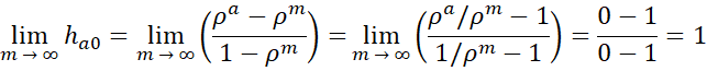
This means that in the long run, Player A will lose all his money. Even in the case where p = q, we have

When does Player B go broke?

Property 2: The probability that one of players will go broke in the gambler’s ruin game is 1. The probability that Player B goes broke is 1 – h_a0 (as described in Property 1).

Proof: Let U = {0, m}. We first prove that h_iU = 1 for any i. The proof is almost identical to the proof of Property 1. The only difference is the impact of the initial condition that h_mU = 1, whereas h_m0 = 0.

When p = .5, as before

h_iU = A + Bi

Using the initial conditions, we obtain

 1 = h_0U = A + B(0) = A

1= h_mU = A + Bm = 1 + Bm

we see that A = 1 and B = 0. Thus

h_iU = A + Bi = 1 + 0 = 1

When p ≠.5

h_iU = A + Bρⁱ

Using the initial conditions, we obtain

 1 = h_0U = A + Bρ⁰ = A + B

1= h_mU = A + Bρ^m = 1 + Bρ^m

Bρ^m = 0

Thus, B = 0 and A = 1, and so

h_iU = A + Bρⁱ = 1 + 0 = 1

Now since 0 and m are both absorbing states, h_i0 + h_im = h_iU = 1. Thus h_im = 1 – h_i0.

Expected duration

Property 3: The expected duration for gambler’s ruin is

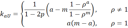
where U = {0, m}.

Proof: Using the approach from Hitting Probabilities, we see that

k_iU = 1 + pk_i+1,U + qk_i-1,U          k_0U = 0     k_mU = 0

This can be expressed as the second-order non-homogeneous difference equation

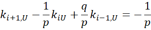
As we saw in the proof of Property 1, the roots of the characteristic equation for this difference equation are again 1 and ρ = q/p. We use the approach described in Second-order Difference Equations to deal with the non-homogeneous component.

Two distinct real roots case

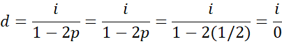
We first note that

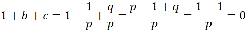
Since this is zero, we, instead, define d as follows:

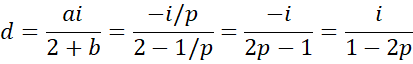
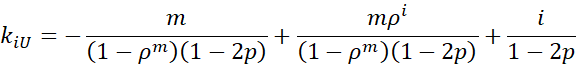
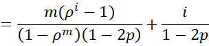
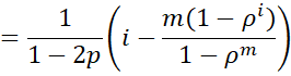
Thus, we can express k_iU as follows

k_iU = A + Bρⁱ – i/(1–2p)

Using the initial conditions, we observe that

0 = k_0U = A + Bρ⁰ – 0/(1–2p) = A + B

Thus, A = –B.

(1 – ρ^m)B = m/(1–2p)

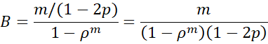
Thus

k_iU = A + Bρⁱ – i/(1–2p)

One root case

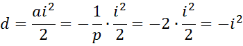
If p = q, then 1 is the only root. Since p = 1/2,

So we need to use the following expression for d

Thus, k_iU can be expressed as

k_iU = A + Bi – i²

Again, we use the initial conditions, as follows:

0 = k_0U = A + B(0) – 0² = A

0 = k_mU = A + B(m) – m² = 0 + Bm – m²

Thus, B = m. Thus, the general solution can be expressed as

k_iU = A + Bi – i² = 0 + m – m² = m(1 – m)

Limiting case

When Player B has a huge cash reserve (e.g. a casino), we can estimate k_aU by using the limit when b → ∞ (or equivalently when m → ∞). Also, suppose that the odds are in favor of Player B (i.e. q > p).

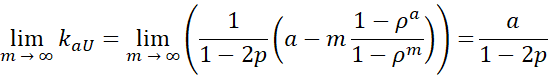
Since q > p, ρ^m → ∞ faster than m → ∞, which is why m(1 – ρ^a)/(1 – ρ^m) → 0.

We conclude that Player A will go broke in an average of a/(q–p) steps.

In the case where p = q = .5 (even odds)

We conclude that although Player A will eventually go broke, it might take a long time to do so.

Worksheet Functions

Starting in Rel 9.9, the Real Statistics Resource Pack will provide the following worksheet functions using Properties 1 and 3:

RuinProb(p, a, b) = probability that player A goes broke, assuming the probability that Player A wins on each round is p, and that he starts with $a and Player B starts with $b.

RuinHits(p, a, b) = # of steps until one of the players goes broke, given that p, a, and b are as above.

Examples

Example 1: Figure 1 shows the probability that Player A goes broke for various p, a, and b values (the prob rows using the RuinProb function). It also shows the expected number of steps until one of the players goes broke (the exp steps rows using the RuinHits function).

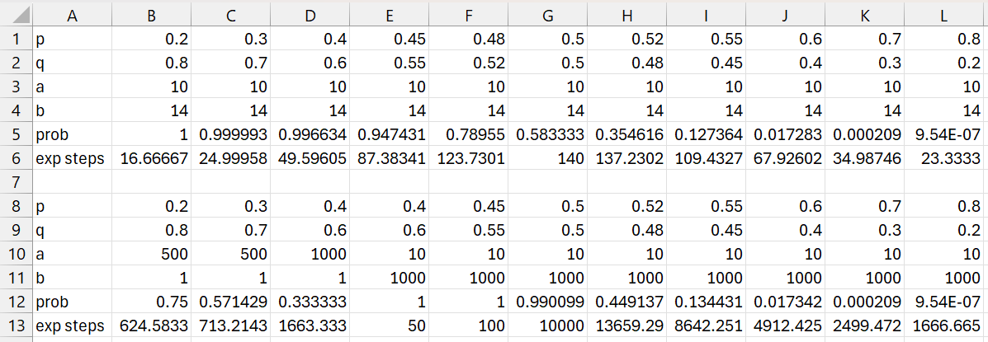
Figure 1 – Gambler’s ruin outcomes

Note that these functions are subject to overflow problems for extreme values. E.g. =RuinProb(.3, 10, 1000) returns the #VALUE! error value. Since =RuinProb(.4, 10, 1000) returns the value 1, clearly the probability that Player A goes broke in the more extreme case where p = .3, a = 10, and b =1,000 is also 1.

Using Hits simulation

We can also use the simulation worksheet function described Hitting Probabilities Real Statistics Support to approximate these values, as well as get additional insight.

Example 2: Use simulation for the case where a = 10, b = 14, and p = .5.

The result is shown in Figure 2.

Figure 2 – Simulation where p = .5

The output from =MarkovSimHit(B2:Z26,11,1,1000,1000) is shown in range AF2:AF3. Note that for the Gambler’s ruin chain, the states run from 0 to where x₀ = a = 10, and then on to m = 10+14 = 24. For MarkovSimHit, the states start at 1, not 0; so we specify the start at 11, instead of 10, and the target value as 1 instead of 0. We see that of the 1,000 simulations, 58.5% (cell AF2) end in Player A going broke. This is pretty close to the 58.33% shown in cell G5 of Figure 1. When Player A goes broke, on average, it takes 120.3 steps (cell AF3).

The output from =MarkovSimHit(B2:Z26,11,{1;25},1000,1000) is shown in range AF5:AF6. Here, {1;25} represents the two absorption states 0 and 24. Note that a semi-colon is used since a column array is expected. The value is close to 1, as expected per Property 3. Note that 1 of the 1,000 simulations (last argument in the formula) exceeded the 1,000 simulation length (second-to-last argument), so that the hit probability is estimated to be .999 (cell AF5) instead of 1. The value 141.341 in cell AF6 is an estimate of k_aU = 140 shown in cell G6 of Figure 1.

Average steps if Player B goes broke

If we use the .5833 and 140 estimates from Figure 1 and the 120.3 estimate from Figure 2, we can obtain an estimate of the average number of steps when Player B goes broke of 167.555, as shown in Figure 3.

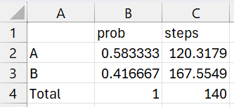
Figure 3 – Average steps when Player B goes broke

Here, we seek the value for cell C3 such that =SUMPRODUCT(B2:B3,C2:C3) is the value in cell C4. This turns out to be 167.555. You can use Excel’s Goal Seek to find this value.

Simulation Worksheet Function

Starting with Rel 9.9, the Real Statistics Resource Pack will provide the following worksheet function:

RuinSim(p, a, b, n, m): performs m simulations, each of length n, of the gambler’s ruin problem, and returns a 6 × 2 column array whose second column contains the following values: the probability that Player A goes broke, the probability that Player B goes broke, the probability that either player goes broke,  the expected number of steps when Player A goes broke, the expected number of steps when Player B goes broke, and the expected number of steps until either player goes broke. The first column contains labels for the entries in the second column.

Examples

Figure 4 uses RuinSim to estimate the probabilities that each player goes broke and the expected number of steps required. You can compare the results in range E2:E7 with those in G5:G6 of Figure 1 or AE2:AF6 of Figure 2. You can compare the results in range K2:K7 with those in E5:E6 of Figure 1.

Similarly, you can compare the results in E9:E15 with those in D12:D13 of Figure 1. Note that you need to set the length of each Markov chain in cell B13 pretty high to obtain a hit probability of 1 in cell E11. Finally, you can compare the results in K9:K15 with those in E12:E13 of Figure 1.

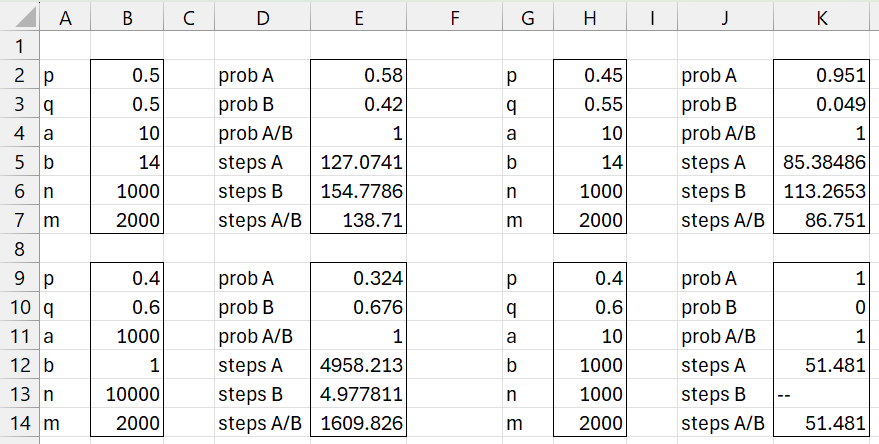
Figure 4 – Gambler’s ruin simulations

Examples Workbook

Click here to download the Excel workbook with the examples described on this webpage.

Links

↑ Markov chains

References

Aldridge, M. (2021) Hitting times. Introduction to Markov Processes
https://mpaldridge.github.io/math2750/S08-hitting-times.html

Norris, J. (2004) Discrete-time Markov chains. Cambridge University Press
https://www.statslab.cam.ac.uk/~jrn10//Markov/

Sargent, T. J., Stachurski, J. (2025) Markov chains: Basic concepts. First course in quantitative economics with Python
https://intro.quantecon.org/markov_chains_I.html