Basic Concepts
Definition 1: A second-order difference equation takes the form
xn = f(n, xn-1, xn-2)
for all positive integers n. A solution is a function g(x, y) such that
xn = g(x0, x1)
By induction on n, such a solution is unique.
Definition 2: A linear second-order difference equation with constant coefficients takes the form
xn = f(n, xn-1, xn-2) = uxn-1 + vxn-2 + w
Alternatively, this can be expressed as
xn+2 + bxn+1 + cxn = a
The difference equation is homogeneous if a = 0.
We start by looking at solutions in the homogeneous case.
Definition 3: The characteristic equation of a second-order difference equation is
y2 + by + c = 0
Solution for homogeneous equations
Property 1: A homogeneous linear second-order difference equation with constant coefficients has a solution based on its characteristic equation, as follows:
If b2 > 4c, then the characteristic equation has two distinct real roots r1 and r2. Any solution of the difference equation takes the form Ar1n + Br2n.
Using the binomial formula, these roots are
![]()
If b2 = 4c, then the characteristic equation has one distinct real root r1 = –b/2. Any solution of the difference equation takes the form (A + Bn)r1n.
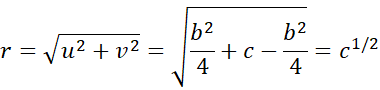
If b2 < 4c, then the characteristic equation has two conjugate complex roots u ± iv where
![]()
Any solution to the homogeneous differential equation takes the form
![]()
Note that
![]()
where
![]()
Alternatively
![]()
Thus
![]()
![]()
Also note
Setting A = C+D and B = (C – D)i, we see that any solution to the homogeneous differential equation takes the form
xn = rn(A cos nθ + B sin nθ)
Using initial values
Property 2: If x0 and x1 are known, we can solve for A and B as follows:
If b2 > 4c, then any solution of the difference equation takes the form Ar1n + Br2n.
x0 = A + B x1 = Ar1 + Br2
Here, x0, x1, r1, and r2 are known. We solve for A and B.
If b2 = 4c, then any solution of the difference equation takes the form (A + Bn)r1n.
x0 = A x1 = (A + Bn)r1
Since x0, x1, and r1 are known, we can solve for A and B.
If b2 < 4c, then any solution of the difference equation takes the form xn = rn(A cos nθ + B sin nθ).
x0 = r0(A cos 0 + B sin 0) = A x1 = r(A cos θ + B sin θ)
Since x0, x1, r, and θ are known, we can solve for A and B.
Solution for non-homogeneous equations
Property 3: If a is not zero, then the solution to the difference equation needs to be modified by adding d to the corresponding homogeneous difference equation solution, where
d = a / (b + c + 1)
If, however, b + c + 1 = 0, then we set
d = an / (b + 2)
provided that b ≠ -2. Otherwise, we set
d = an2 / 2
Let d0 be the value of d when n = 0, and d1 be the value of d when n = 1. When there are two distinct real roots, clearly d0 = d1 = d. For the other two cases, d0 = 0.
We also need to modify the approach for finding the A and B coefficients as follows:
If b2 > 4c, then any solution of the difference equation takes the form Ar1n + Br2n + d.
x0 = A + B + d0 x1 = Ar1 + Br2 + d1
If b2 = 4c, then any solution of the difference equation takes the form (A + Bn)r1n + d.
x0 = A + d0 x1 = (A + Bn)r1 + d1
If b2 < 4c, then any solution of the difference equation takes the form xn = rn(A cos nθ + B sin nθ) + d.
x0 = A+ d0 x1 = r(A cos θ + B sin θ) + d1
Convergence
Definition 4: A steady-state is achieved if the sequence xn converges, i.e. the limit of xn exists as n → ∞.
Property 4: The sequence converges provided
If two distinct real roots: |r1| < 1, |r2| < 1
If one real root: |r1| < 1
If two complex roots: r = √c < 1
Alternatively, the sequence converges if all the following conditions hold:
1 + b + c > 0 1 – b + c > 0 c < 1
Examples and worksheet functions
Click here for examples and Real Statistics worksheet functions.
Links
↑ First-order difference equations
References
Osborne, M. J. (2025) Second-order difference equations
https://mjo.osborne.economics.utoronto.ca/index.php/tutorial/index/1/sod/t
Dowling, E. T. (1980) Introduction to mathematical economics. 3rd ed. Schaum’s Outline
https://ugess3.wordpress.com/wp-content/uploads/2015/08/schaum_introduction_to_mathematical_economics.pdf
Kumar, A. (2008) Linear, second-order difference equations
No longer available online