Objective
We now expand on the concepts described in Second-order Difference Equations by providing illustrative examples and Excel worksheet functions.
Examples: real distinct roots
Example 1:
xn+2 – 10xn+1 + 16xn = 14
x0 = 5 x1 = 20
Homogeneous equation
The roots are
![]()
xn = A ⋅ 2n + B ⋅ 8n
Non-homogeneous equation
1 + b + c = 1 – 10 + 16 = 7
d = a/(1+b+c) = 14/7 = 2
xn = A ⋅ 2n + B ⋅ 8n + 2
Using the initial values
5 = x0 = A ⋅ 20 + B ⋅ 80 + 2 = A + B + 2
20 = x1 = A ⋅ 21 + B ⋅ 81 + 2 = 2A + 8B + 2
Thus
A + B = 3
A + 4B = 9
This means that
A = 1 B = 2
We now check the results
x0 = 1 ⋅ 20 + 2 ⋅ 80 + 2 = 1 + 2 + 2 = 5
x1 = 1 ⋅ 21 + 2 ⋅ 81 + 2 = 2 + 16 + 2 = 20
These results are consistent with the stated initial values. We now check x2
x2 = 1 ⋅ 22 + 2 ⋅ 82 + 2 = 4 + 128 + 2 = 134
which is consistent with the original difference equation, namely
xn+2 – 10xn+1 + 16xn = 14
134 – 10(20) + 16(5) = 134 – 200 + 80 = 14
Example 2:
xn+2 + xn+1 – 2xn = 3
x0 = 1 x1 = 2
Homogeneous equation
The roots are
![]()
xn = A ⋅ (–2)n + B ⋅ 1n = (–2)n A + B
Non-homogeneous equation
1 + b + c = 1 + 1 – 2 = 0
![]()
xn = (–2)n A + B + n
Using the initial values
1 = x0 = (–2)0 A + B + 0 = A + B
2 = x1 = (–2)1 A + B + 1 = –2A + B + 1
Thus
A = 0 B = 1
Hence
xn = 1 + n
Example: one real root
Example 3:
xn+2– 2xn+1 + xn = 8
x0 = –1 x1 = 5
Homogeneous equation
The roots are
![]()
xn = (A + nB)1n = A + nB
Non-homogeneous equation
1 + b + c = 1 – 2 + 1 = 0 b = –2
![]()
xn = A + nB + 4n2
Using the initial values
–1 = x0 = A + 0⋅B + 4⋅02 = A
5 = x1= A + 1⋅B + 4⋅12 = A + B + 4
Thus
A = –1 B = 2
xn = –1 + 2n + 4n2
Examples: complex roots
Example 4:
xn+2 – xn+1 + xn = 0
x0 = –1 x1 = 2
Homogeneous equation
The roots are
![]()
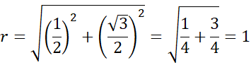
cos θ = (1/2)/1 = 1/2 → θ = acos(1/2) = π/3
xn = rn(A cos nθ + B sin nθ)
![]()
Using the initial values
–1 = x0 = A cos 0 + B sin 0 = A
![]()
Thus
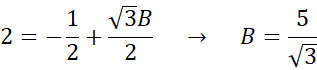
![]()
We now check these results as follows:
![]()
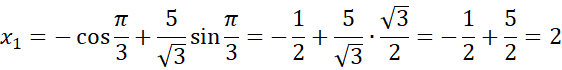
These results are consistent with the stated initial values.
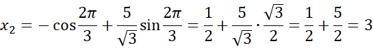
which is consistent with the original difference equation, namely
xn+2 – xn+1 + xn = 0
3 – 2 – 1 = 0
Example 5:
xn + 4xn-2 = 20
x0 = 6 x1 = 5
Homogeneous equation
The roots are
![]()
![]()
cos θ = 0/2 = 0 → θ = acos 0 = π/2
xn = rn(A cos nθ + B sin nθ)
![]()
Non-homogeneous equation
1 + b + c = 1 – 0 + 4 = 5
d = a/(1+b+c) = 20/5 = 4
![]()
Using initial values, we obtain
6 = x0 = r0(A cos 0 + B sin 0) + 4 = A + 4 → A = 2
![]()
Thus
2B + 4 = 5 → B = 1/2
We now check the results
x0 = r0(2 cos 0 + 1/2 sin 0) + 4 = (2 + 0) + 4 = 6
![]()
These results are consistent with the stated initial values.
![]()
which is consistent with the original difference equation, namely
xn + 4xn-2 = 20
–4 + 4(6) = 20
Worksheet Functions
Starting with Rel 9.9, the Real Statistics Resource Pack will provide the following worksheet function:
DiffEqn2X(a, b, c, x0, x1): returns an 8 × 2 array with the following values in column 2: d, multiplier of d (none = 1, n, or n-sq), root1, root2, A, B, formula for xn, stability (converge or diverge). Column 1 contains the appropriate labels. If the roots are complex, then root1 and root2 are replaced by the amplitude r and angle θ. x0 and x1 default to 0.
The output from DiffEqnX(B2, B3, B4, B5, B6) for Example 1 is shown in Figure 1.
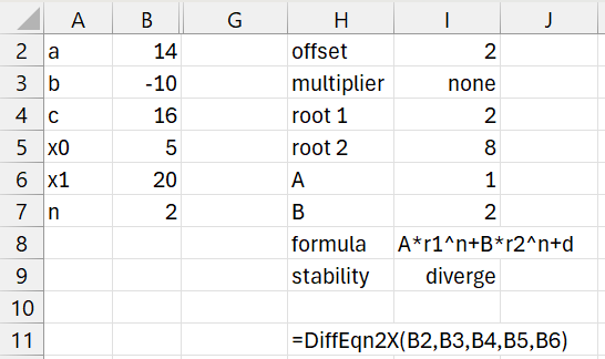
Figure 1 – Example 1
The output for Example 3 is shown in Figure 2.
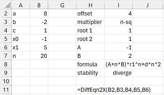
Figure 2 – Example 3
The output for Example 4 is shown in Figure 3.
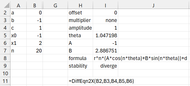
Figure 3 – Example 4
In addition, Real Statistics provides the following function:
DiffEqn2(a, b, c, x0, x1, n, prop) = xn
If prop = TRUE (default), then Properties 1, 2, and 3 from Second-order Difference Equations are used. Otherwise, the function repeatedly uses the formula
xn = a – bxn-1 – cxn-2
together with the initial values x0 and x1.
Example 6: Find x20 for the difference equation (Example 2)
xn+2 + xn+1 – 2xn = 3
x1 = 1 x2 = 2
Using the formula =DiffEqn2(3,1,-2,1,2,20), we obtain the value x20 = 21. We obtain the same result using the formula =DiffEqn2(3,1,-2,1,2,20,FALSE).
Links
↑ First-order difference equations
↑ Second-order difference equations
References
Osborne, M. J. (2025) Second-order difference equations
https://mjo.osborne.economics.utoronto.ca/index.php/tutorial/index/1/sod/t
Dowling, E. T. (1980) Introduction to mathematical economics. 3rd ed. Schaum’s Outline
https://ugess3.wordpress.com/wp-content/uploads/2015/08/schaum_introduction_to_mathematical_economics.pdf
Kumar, A. (2008) Linear, second-order difference equations
No longer available online