Hitting Probabilities

Basic Concepts

Definition 1: For a Markov chain x_n, the hitting time is the time to hit a subset of states A, i.e.

If the Markov chain never hits A, then H_A = ∞. If A is a closed class, then the hitting time is also called the absorption time.

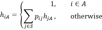
The hitting probability for state i to a set of states A is

We can also define

Thus

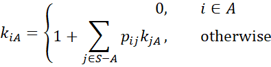
The expected (aka mean) hitting time is

Clearly, k_iA < ∞ only if h_iA = 1.

If A consists of a single state j, then we denote H_A, h_iA, and k_iA by H_j, h_ij and k_ij, respectively.

Definition 2: For a Markov chain x_n, the return time T_A is the time to hit a subset of states A, i.e.

T_A = min {n : x_n ∈ A and n > 0}

If the Markov chain never returns to A, then T_A < ∞.

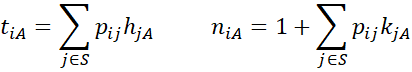
The expected (aka mean) return time is

n_iA = E[T_A | x₀ = i]

Clearly, n_iA < ∞ only if t_iA = 1.

If A consists of a single state j, then we denote T_A, t_iA, and n_iA by T_j, t_ij and n_ij, respectively. Also, we use t_i and n_i for t_ii and n_ii, respectively.

Hitting probability examples

Example 1: Find h₁₂ for the Markov chain with the transition matrix

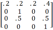
We first note

h₁₂ = p₁₁h₁₂ + p₁₂h₂₂ + p₁₃h₃₂ + p₁₄h₄₂ 

h₁₂ = .2 h₁₂ + .2 h₂₂ + .2 h₃₂ + .4 h₄₂ 

Thus, to find h₁₂ we also need to find h₂₂, h₃₂, h₄₂. We first note that h₂₂ = 1 by definition, and h₄₂ = 0 since 4 is an absorbing state. We also observe that

h₃₂ = p₃₁h₁₂ + p₃₂h₂₂ + p₃₃h₃₂ + p₃₄h₄₂ 

h₃₂ = .5 h₂₂ + .5 h₄₂ = .5(1) + .5(0) = .5

Thus

h₁₂ = .2 h₁₂ + .2 h₂₂ + .2 h₃₂ + .4 h₄₂ = .2 h₁₂ + .2(1) + .2(.5) + .4(0)

h₁₂ = .2 h₁₂ + .2 + .1 = .2 h₁₂ + .3

Solving for h₁₂, we have

.8h₁₂ = .3

and so

h₁₂ = 3/8

Example 2: Find h₁₃ for the Markov chain with the transition matrix

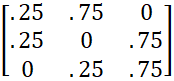
This time we observe that

h₁₃ = p₁₁h₁₃ + p₁₂h₂₃ + p₁₃h₃₃ 

h₁₃ = .25 h₁₃ + .75 h₂₃ + 0 h₃₃

Hence

.75 h₁₃ = .75 h₂₃

h₁₃ = h₂₃

But

h₂₃ = p₂₁h₁₃ + p₂₂h₂₃ + p₂₃h₃₃ 

h₂₃ = .25 h₁₃ + 0 h₂₃ + .75 h₃₃

h₂₃ = .25 h₂₃ + .75 ⋅ 1

.75 h₂₃ = .75

h₁₃ = h₂₃ = 1

Example 3: Find h_1A, h_2A, h_3A, and h_4A where A = {1,3} for the Markov chain with the transition matrix

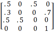
Clearly, h_1A = h_3A = 1 since 1, 3 are in A. Also, h_4A = 0 since 4 is an absorbing state.

h_2A = p₂₁h_1A + p₂₂h_2A + p₂₃h_3A + p₂₄h_4A

h_2A = .3 (1) + 0 h_2A + 0(1)  + .7 (0) = .3

Expected hitting time examples

Example 4: Find k₁₃ for the Markov chain in Example 2.

The analysis is similar to that of h₁₃, but this time we need to add 1 since the first step takes one time unit.

k₁₃ = 1 + p₁₁k₁₃ + p₁₂k₂₃ + p₁₃k₃₃ 

k₁₃ = 1 + .25 k₁₃ + .75 k₂₃ + 0 k₃₃

Thus

. 75 k₁₃ = 1 + .75 k₂₃

k₁₃ = 4/3 + k₂₃

Similarly

k₂₃ = 1 + p₂₁k₁₃ + p₂₂k₂₃ + p₂₃k₃₃ 

k₂₃ = 1 + .25 k₁₃ + 0 k₂₃ + .75 k₃₃

k₂₃ = 1 + .25 k₁₃

since k₃₃ = 0. From the earlier result, we observe that

k₁₃ = 4/3 + k₂₃ = 4/3 + 1 + .25 k₁₃

 .75 k₁₃ = 7/3

k₁₃ = 7/3 ⋅ 4/3 = 28/9 ≈ 3.11111

Example 5: Find k₃₂ for the Markov chain in Example 1.

First note that k₂₂ = 0 since the chain is already at the destination. But k₄₂ = ∞ since once in state 4, you can never enter state 2. But p₃₄ ≠ 0, and so you can go from state 3 to state 4. Thus

k₃₂ = 1 + p₃₁k₁₂ + p₃₂k₂₂ + p₃₃k₃₂ + p₃₄k₄₂ 

k₃₂ = 1 + 0 ⋅ k₁₂ + .5 ⋅ 0 + 0 ⋅ h₃₂ + .5 ⋅ ∞ = ∞

This is not surprising since h₃₂ ≠ 1.

Properties

Property 1:

If there are multiple solutions, the hitting probabilities are the smallest such non-negative solutions.

Property 2:

If there are multiple solutions, the expected hit times are the smallest such non-negative solutions.

Property 3:

Real Statistics support

Click here for a description of Real Statistics support for hitting probabilities.

More examples

Click here for a description of the Gambler’s Ruin problem.

Click here for a description of Random Walk Markov chains.

Links

↑ Markov chains

References

Aldridge, M. (2021) Hitting times. Introduction to Markov Processes
https://mpaldridge.github.io/math2750/S08-hitting-times.html

Norris, J. (2004) Discrete-time Markov chains. Cambridge University Press
https://www.statslab.cam.ac.uk/~jrn10//Markov/

Sargent, T. J., Stachurski, J. (2025) Markov chains: Basic concepts. First course in quantitative economics with Python
https://intro.quantecon.org/markov_chains_I.html

Tolver, A. (2016) Introduction to Markov chains
https://www.math.ku.dk/bibliotek/arkivet/noter/stoknoter.pdf

Chao, J. C. (2020) Markov chains
http://econweb.umd.edu/~chao/Teaching/Econ721/Econ721_Lecture_on_Markov_Chains.pdf