Random Walk Markov Chains

Basic Concepts

Random walks are defined similarly to the gambler’s ruin. The difference is that the set of states is the set of all integers, an infinite set. For any states i and j, the transition probabilities are

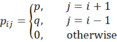
Here, p and q take numeric values 0 < p, q < 1 with p+q = 1.

Example 1: What is the probability that x₂ = 2, starting with x₀ = 0? This can only happen with two steps to the right, namely p² ₀₂ = p²

Example 2: What is the probability that x₂ = -1, starting with x₀ = 0? This can happen in three different ways: (1) 1 step to the right and 2 steps to the left, (2) 2 steps to the left and 1 step to the right, and (3) 1 step left, 1 step right, and 1 step left. Thus, the probability is p³_0,-1 = p*q² + q²*p + q*p*q = 3*p*q².

Mean and variance

A random walk can be defined by

where the z_i are independent, identically distributed random variables with distribution P(z = 1) = p and P(z = –1) = q. The mean is μ = E[z] = 1 · p + (–1) · q = p–q.

Assuming x₀ = 0, the expected value for x_n is

The variance of z is

var(z) = E[(z – μ)²] = p(1 – (p–q))² + q(–1 – (p–q))²

= p((p+q) – (p–q))² + q(–(p+q) – (p–q))²

= p(–2q)² + q(–2p)² = 4pq² + 4p²q = 4pq(q+p) = 4pq

Thus

Probability x_n = i

Let y_n = the number of times the random walk went to the right in n steps. Then y_n ∼ Bin(n, p). Thus

P(y_n = k) = C(n, k) p^k q^n-k

If y_n = k then x_n = k – (n–k) = 2k–n. Hence

Note that n+i must be divisible by 2. Thus, they must both be even or both odd. Otherwise,  P(x_n = i) = 0.

Distribution worksheet function

Starting with Rel 9.9, the Real Statistics Resource Pack will provide the following worksheet function (in two formats):

RandWalkDist(i, n, p) = P(x_n = i) for the random walk Markov chain with the stated value of p

RandWalkDist(i, n, p, j) = the sum of P(x_n = k) for k = i to j, for the random walk Markov chain with the stated value of p. If j < i, then the roles of i and j are reversed.

Examples

Figure 1 provides some examples of the use of the RandWalkDist function. Column B lists the values of P(x₁₀ = i) when p = .5 for various values of i. Column C lists the values of P(x₉ = i).

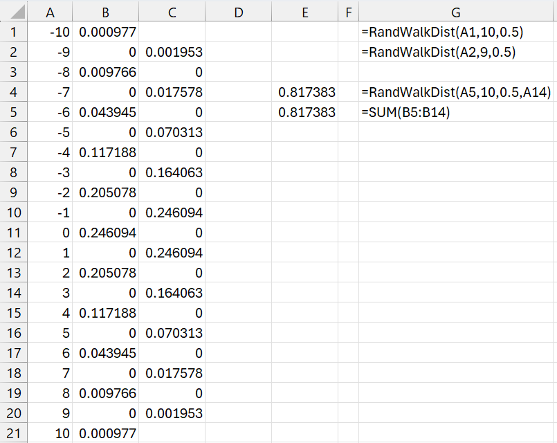
Figure 1 – Random walk distribution values

Expected distance

Let the distance from the origin at step n be d_n = |x_n|. If p = q, thenThe proof is described in Binomial Distribution and Random Walks. The proof is also provided in the Wolfram reference below. 

Hitting probabilities

Assuming that the probability of taking a step to the right is p and the probability of taking a step to the left is q, we see that

h_i0 = ph_i+1,0 + qh_i-1,0          h₀₀ = 1

This is the homogeneous second-order linear difference equation

As we observe for the gambler’s ruin, the roots are 1 and ρ = (1–p)/p = q/p. When p ≠ .5

h_i0 = A + Bρⁱ          h₀₀ = 1

1 = h₀₀ = A + Bρ⁰ = A + B

h_i0 = (1 – B)+ Bρⁱ = 1 + B(ρⁱ – 1)

Estimating B

This time, we don’t have a second initial value to calculate B. Suppose i > 0. If ρ > 1 (i.e. p < .5), then ρⁱ → ∞ as i → ∞. If B < 0, then for i big enough, eventually h_i0 becomes negative, which is impossible for a probability. If B > 0. Then h_i0 > 1, which is also impossible. Thus, B = 0 and h_i0 = 1.

If, instead, ρ < 1, then ρⁱ → 0 as i → ∞. In which case, h_i0 = 1 + B(ρⁱ – 1) → 1 + B, which forces B to take a value between 0 and 1, inclusive. The minimum solution (per Property 1 of Hitting Probabilities) occurs when B = 1. In this case,

h_i0 = 1 + B(ρⁱ – 1) = ρⁱ

If i < 0, then the same logic applies with roles of p and q reversed.

When ρ = 1 (i.e. p = .5),

h_i0 = 1 + Bi

Since 0 ≤ h_i0 ≤ 1, Bi ≤ 0. Thus, for i > 0, B ≤ 0. But for any negative value of B, for i large enough, eventually, 1+Bi < 0, which is impossible. Thus, B = 0, and so h_i0 = 1. If i < 0, then B ≥ 0. If B is positive, then for i large enough in absolute value, h_i0 < 0. Thus, again B = 0, and h_i0 = 1.

Results

In conclusion:

h_i0 = 1 if (a) i = 0 or p = .5, (b) i > 0 and p < .5, or (c) i < 0 and p > .5

h_i0 = ρⁱ if (d) i > 0 and p > .5, or (e) i < 0 and p < .5

Hitting times

As we observed above, for any p ≠ .5, there are i such that h_i0 < 1. Thus, k_i0 = ∞.

Suppose p = .5. As we showed above, h_i0 = 1 for all i. To estimate the hit time, we use the equation

k_i0 = 1 + pk_i+1,0 + qk_i-1,0          k₀₀ = 0

k_i0 = 1 + .5 k_i+1,0 + .5 k_i-1,0         k₀₀ = 0

As we observe in Gambler’s Ruin, the solution to this non-homogeneous second-order linear difference equation takes the form

k_i0 = A + Bi – i²

Using the initial condition, we obtain

0 = k₀₀ = A + B(0) – 0² = A

Thus

k_i0 = Bi – i² = (B – i)i

No matter what non-negative value we choose for B, for any i > B, we see that k_i0 < 0, which is a contradiction. Similarly, for any negative B, k_i0 < 0 for any i < B. We conclude that there is no solution to the difference equation; i.e. k_i0 = ∞.

Return probabilities

By Property 4 of Hitting Probabilities

t₀ = p₀₁h_1,0 + p_0,-1h_-1,0

= ph_1,0 + qh_-1,0

If p = q = .5, we just saw that h_i0 = 1 for all i. Thus

t₀ = p + q = 1

If p < .5 then h_i0 = 1 for i > 0, and h_i0 = (q/p)ⁱ for i < 0. Thus

t₀ = p + q(q/p)^-1 = p + p = 2p < 1

If p > .5 then h_i0 = 1 for i < 0, and h_i0 = (q/p)ⁱ for i > 0. Thus

t₀ = p(q/p)¹ + q = q + q = 2q < 1

Return times

If p ≠ .5, there is some probability that we won’t return to state 0. Thus, the return time n₀ = ∞.

If p = .5, then we are certain to return to state 0. By Property 4 of Hitting Probabilities

n₀ = 1 + p₀₁k_1,0 + p_0,-1k_-1,0

= 1 + pk_1,0 + qk_-1,0 = 1 + .5(∞) + .5(∞) = ∞

In this case, while we are certain that the chain returns to 0, it can can a long time for it to do so.

Simulation worksheet function

Starting with Rel 9.9, the Real Statistics Resource Pack will provide the following function that simulates a random walk of length n, where p = the probability of one step to the right and start is the starting state (default 0).

RandWalkSim(p, n, start, bound1, bound2): returns an n × 1 array with the states of the random walk simulation.

If bound1 or bound2 is specified, then when either state is entered, the Markov chain stays there (absorption state). Using these arguments provides a way of simulating a gambler’s ruin chain (see example below).

Examples

We can use the formula =RandWalkSim(.4, 24) to create a random walk of length 25, as shown in columns A and B of Figure 2.

We can also simulate gambler’s ruin, as shown in columns D, E, and F. Range D1:D24 contains the formula =RandWalkSim(.5, 24, 10, 0, 24). Here, p = .5, a = 10, and m = 24 (using the terminology from Gambler’s Ruin). Ranges E1:E24 and F1:F24 contain the same formula, except that p = .5 is replaced by p = .8 and p = .2, respectively. Note that Player B goes broke in column E and Player A goes broke in column F.

Column H shows a different version of gambler’s ruin using the formula =RandWalkSim(.2, 24, , -10, 14). This time, the game starts at 0, and Player A goes broke if he loses $10 (the -10 argument) and Player B goes broke if the random walk hits 14 (i.e. Player B loses $14).

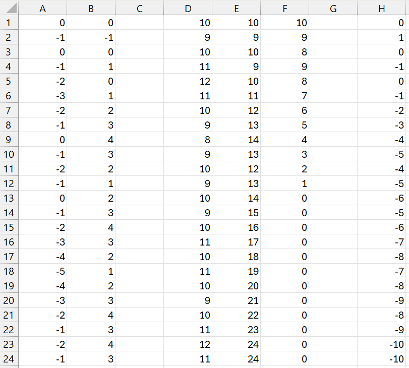
Figure 2 – RandWalkSim examples

Return simulation function

Starting with Rel 9.9, the Real Statistics Resource Pack will provide the following function that simulates m random walks, each of maximum length n, where p = the probability of one step to the right and start is the starting state (default 0).

RandWalkSimReturn(p, n, m, start): returns a 4 × 2 array whose second column contains (1) the probability that the random walk returns to start, (2) the expected number of steps needed to return to start, (3) the average farthest distance from start when there is a return to start, and (4) the average farthest distance from start when there isn’t a return to start. The first column contains labels for the second column.

Examples

Figure 3 contains some examples of the use of the RandWalkSimReturn function. E.g. range A5:B8 contains the formula =RandWalkSimReturn (B2,B3,B4) and range C5:C8 contains the formula =SUBMATRIX(RandWalkSimReturn(C2,C3,C4),,2).

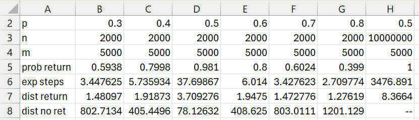
Figure 3 – RandWalkSimReturn examples

Examples Workbook

Click here to download the Excel workbook with the examples described on this webpage.

Links

↑ Markov chains

References

Aldridge, M. (2021) Hitting times. Introduction to Markov Processes
https://mpaldridge.github.io/math2750/S08-hitting-times.html

Norris, J. (2004) Discrete-time Markov chains. Cambridge University Press
https://www.statslab.cam.ac.uk/~jrn10//Markov/

Sargent, T. J., Stachurski, J. (2025) Markov chains: Basic concepts. First course in quantitative economics with Python
https://intro.quantecon.org/markov_chains_I.html

Wolfram (2026) Random walk – 1 dimensional
https://mathworld.wolfram.com/RandomWalk1-Dimensional.html