We now describe worksheet functions in the Real Statistics Resource Pack that support the Baum-Welch algorithm for Hidden Markov Models.
Worksheet Functions
The Real Statistics Resource Pack provides the following functions where Rp is a k × k transition matrix, Rd is a k × 1 initial distribution array, Rq is a k × m emission matrix, and Ro is an n × 1 array of observations.
HMM_Rho(Rp, Rd, Rq, Ro): returns a revised k × k transition matrix using one iteration of the Baum-Welch algorithm
HMM_Pi(Rp, Rd, Rq, Ro): returns a revised k × 1 distribution array using one iteration of the Baum-Welch algorithm
HMM_Kappa(Rp, Rd, Rq, Ro): returns a revised k × m emission matrix using one iteration of the Baum-Welch algorithm
We can obtain the results in Figure 4 of HMM Baum-Welch Algorithm by inserting the array formula =HMM_Rho(B3:C4,D3:D4,B7:D8,F3:F22) in range B12:C13, =HMM_Pi(B3:C4,D3:D4,B7:D8,F3:F22) in range D12:D13, and =HMM_Kappa(B3:C4,D3:D4,B7:D8,F3:F22) in B16:D17.
Iterative Approach
So far, we have described only the first iteration of the Baum-Welch algorithm. We can repeatedly use these three worksheet functions until convergence, as illustrated in Figure 1. The figure shows only the first three and last three of 49 iterations. Note too that the last 9 observations in range K2:21 are cut off.
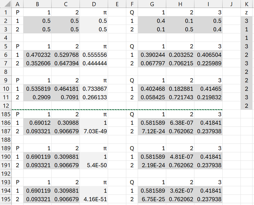
Figure 1 – Baum-Welch iterations
It appears that we have convergence to at least 6 significant figures, resulting in the matrices displayed in Figure 2.

Figure 2 – Baum-Welch parameters
Worksheet Functions
The Real Statistics Resource Pack provides the following function where Rp is the initial k × k transition matrix, Rd is a k × 1 initial distribution array, Rq is a k × m initial emission matrix, and Ro is an n × 1 array of observations. iter = the maximum number of iterations (default 100), although convergence is deemed to be reached when no parameter changes by more than prec (default .0000001) in absolute value.
HMM_Baum(Rp, Rd, Rq, Ro, iter, prec): returns a k × k+m+2 array, where the first k columns represent the transition matrix using the Baum-Welch algorithm, the next column represents the distribution array, and the next m columns represent the emission matrix. The first two rows of the last column display the number of iterations and the size of the largest change in any parameter, in absolute value.
For Example 1 of HMM Baum-Welch Algorithm, we obtain the results shown in Figure 3 when we insert the formula
=HMM_Baum(B2:C3,D2:D3,G2:I3,K2:K21)
in range N3:T4.
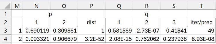
Figure 3 – Baum-Welch formula
Example 1: For the Hidden Markov Model from Example 1 of Viterbi Algorithm for HMM, we generated a 25-element sequence of observations, as shown in column I of Figure 4, using the HMM_Sim worksheet function. Using the HMM_Baum function, we then estimated the HMM parameters that fit these observations, as shown on the right side of Figure 4. Note that we increased the number of iterations from the default to get the desired level of precision.
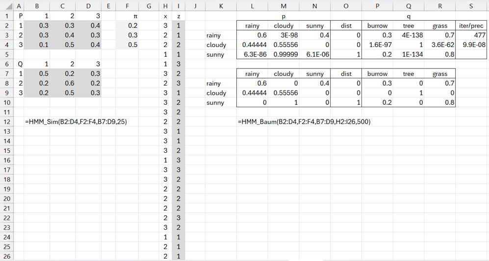
Figure 4 – Baum-Welch formula using simulated data
Multiple observation sequences
We can also use the Baum-Welch algorithm with multiple observation sequences. In this case, on each iteration we perform the algorithm on each observation sequence and then use the average of the resulting transition matrices, and, similarly, the average of the distribution vectors and emission matrices.
Worksheet Functions
The Real Statistics Resource Pack provides the following functions: HMM_RhoX, HMM_PiX, HMM_KappaX, and HMM_BaumX. These functions are identical to HMM_Rho, HMM_Pi, HMM_Kappa, and HMM_Baum, described previously, except that now Ro can be an n × h matrix of observations, where h ≥ 1.
Example 2: Use the Baum-Welch algorithm to estimate HMM parameters based on the ten observation sequences shown in range K2:T11 of Figure 5, using the initial transition, distribution, and emission matrices from Example 1.
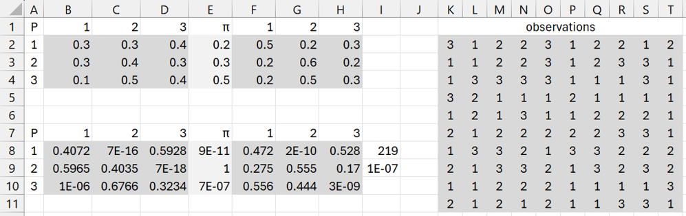
Figure 5 – Baum-Welch with multiple observation sequences
Links
Examples Workbook
Click here to download the Excel workbook with the examples described on this webpage.
References
Frazzoli, E. (2010) Intro to Hidden Markov Models
https://ocw.mit.edu/courses/16-410-principles-of-autonomy-and-decision-making-fall-2010/55e488318190f148c4ed211e2c96bada_MIT16_410F10_lec20.pdf
Frazzoli, E. (2010) Intro to Hidden Markov Models, the Baum-Welch algorithm
https://ocw.mit.edu/courses/16-410-principles-of-autonomy-and-decision-making-fall-2010/2ebbc8cc4bc9adc3418a572a17331f63_MIT16_410F10_lec21.pdf