HMM Baum-Welch Algorithm

Objective

We now focus on finding the most likely set of parameters of an HMM that generates a sequence of observations z₁, …, z_n. Here, the set of parameters encompasses the transition matrix, initial distribution, and emission matrix.

We do this using the Baum-Welch algorithm.

Baum-Welch Algorithm

To explain the Baum-Welch algorithm, we define the following:

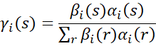
γ_i(s) = probability that the HMM is in state s at time i given observations z_1:i = z₁, …, z_i 

ρ_i(r, s) = probability that the HMM is in state r at time i and s at time i+1 given observations z_1:i

Note that the denominators of γ_i(s) and ρ_i(r, s) are the same, and equal P(z_1:i).

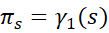
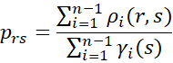
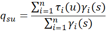
Once we calculate the γ_i(s) and ρ_i(r, s), we can update the parameters of the HMM as follows:

where

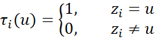
The algorithm uses an EM approach (see EM Algorithm).

We start by initializing the HMM parameters (using guesses). On each step, we calculate the γ_i(s) and ρ_i(r, s) values, and then use these values to update the HMM parameters.

Example

Example 1: Find the HMM with two hidden states that best produces the 20 observations shown in range K3:K22 of Figure 1.

We initialize the P, π, and Q as shown on the left side of Figure 1.

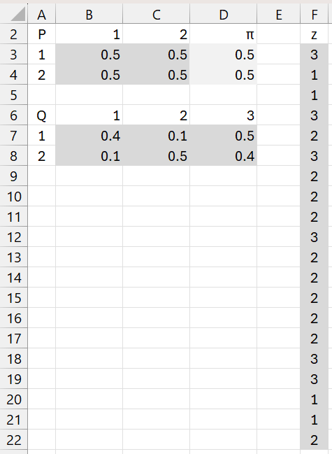
Figure 1 – Baum-Welch algorithm (part 1)

We next calculate the α_i(s) and β_i(s) values shown on the left side of Figure 2, as described in HMM Forward/Backward Algorithms, including using the HMM_Forward and HMM_Backward worksheet functions.

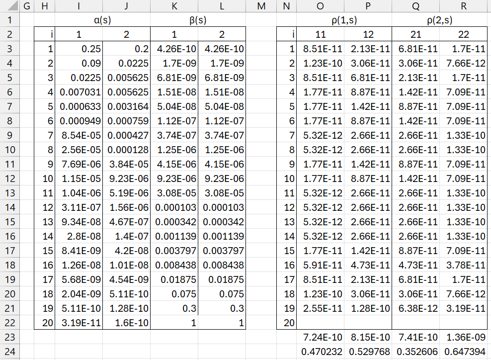
Figure 2 – Baum-Welch algorithm (part 2)

We obtain the numerators of the ρ_i(r,s) expressions, as shown on the right side of Figure 2. Here, we insert the formulas =I3*K4*$B$3*INDEX($B$7:$D$8,1,F4), =I3*L4*$C$3*INDEX($B$7:$D$8,2,F4), =J3*K4*$B$4*INDEX($B$7:$D$8,1,F4), and =J3*L4*$C$4*INDEX($B$7:$D$8,2,F4) in cells O3, P3, Q3, and R3, highlight range O3:R21, and press Ctrl-D.

We now place the formula =SUM(O3:O21) in cell O23, highlight range O23:R23, and press Ctrl-R. Finally, we place the formulas =O23/(O23+P23), =P23/(O23+P23), =Q23/(Q23+R23), and =R23/(Q23+R23), in cells O24, P24, Q24, and R24, respectively. The values in range O24:R24 become the new transition matrix values.

We calculate the revised emission matrix as shown in Figure 3.

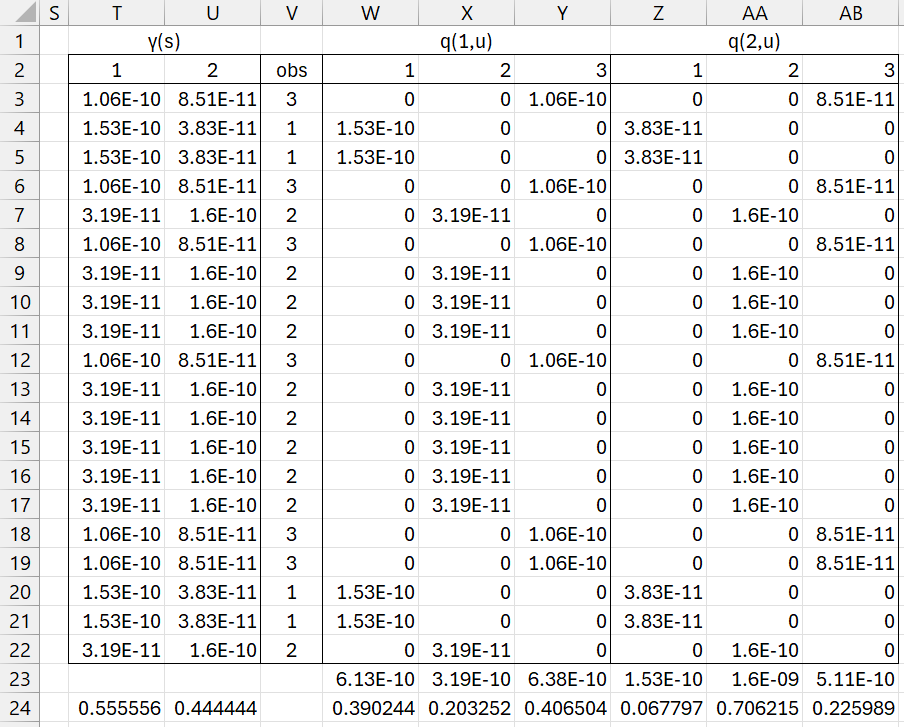
Figure 3 – Baum-Welch algorithm (part 3)

Here, the γ_i(s) values are shown on the left side of the figure. We accomplish this by inserting the formula =I4*K4 in cell T3, highlighting range T3:U22, and pressing Ctrl-R and Ctrl-D. Note too that the value in each row of column T can also be calculated as the sum of the row values in columns O and P of Figure 2. Similarly, the value in each row of column U can also be calculated as the sum of the row values in columns Q and R.

The first row of these gamma values can be used to create the revised distribution array, as shown in range T24:U24. Here, cell T24 contains the formula =T3/($T3+$U3) and cell U24 contains =U3/($T3+$U3).

Column V is copied from column K and is used to calculate the revised emission matrix values, as shown on the right side of Figure 5. Here, we place the formula =IF($V3=W$2,$T3,0) in cell W3, highlight range W3:Y22, and press Ctrl-R and Crtl-D. Next, calculate the sums by placing =SUM(W3:W22) in cell W23, highlighting range W23:Y23, and pressing Ctrl-R. Finally, we calculate the first row of the revised emission matrix by inserting =W23/SUM($W23:$Y23) in cell W24, highlighting range W24:Y24, and pressing Ctrl-R. We obtain the second row of the revised emission matrix, shown in range Z24:AB24, similarly using the values in column U.

We now transfer the results of these calculations into revised HMM parameter matrices, as shown in Figure 4.

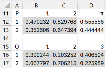
Figure 4 – Revised parameters

Here, range B12:C13 contains the array formula =TRANSPOSE(RESHAPES(O24:R24,2)), D12:D13 contains =TRANSPOSE(T24:U24), and B16:D17 contains =TRANSPOSE(RESHAPES(W24:AB24,3,2)).

Real Statistics Support

Click here to learn about Excel worksheet functions provided by the Real Statistics Resource Pack in support of the Baum-Welch algorithm. Includes additional examples.

Links

↑ Hidden Markov models

Examples Workbook

Click here to download the Excel workbook with the examples described on this webpage.

References

Frazzoli, E. (2010) Intro to Hidden Markov Models
https://ocw.mit.edu/courses/16-410-principles-of-autonomy-and-decision-making-fall-2010/55e488318190f148c4ed211e2c96bada_MIT16_410F10_lec20.pdf

Frazzoli, E. (2010) Intro to Hidden Markov Models, the Baum-Welch algorithm
https://ocw.mit.edu/courses/16-410-principles-of-autonomy-and-decision-making-fall-2010/2ebbc8cc4bc9adc3418a572a17331f63_MIT16_410F10_lec21.pdf