Examples
Example 1: Carry out the analysis for Example 1 of Basic Concepts of ANCOVA using a regression analysis approach.
Our objective is to analyze the effect of teaching method, but without the confounding effect of family income (the covariate). We do this using regression analysis. As we have done several times (see ANOVA using Regression), we use dummy variables for the treatments (i.e. the training methods in this example). We choose the following coding:
t1 = 1 if Method 1 and = 0 otherwise
t2 = 1 if Method 2 and = 0 otherwise
t3 = 1 if Method 3 and = 0 otherwise
We also use the following variables:
y = reading score
x = family income (covariate)
Thus the data from Figure 1 of Basic Concepts of ANCOVA takes the form for regression analysis shown in Figure 1.

Figure 1 – Data for Example 1 along with dummy variables
Different Regression Models
Now we define the following regression models:
-
- Complete model (y, x, t, x*t) – all the variables are used, interaction between treatments and income is modeled
- Full model (y, x, t) – all the variables are used, interaction of treatment with income is not modeled
- Partial model (y, t ) – only reading scores and treatments are used
- Partial model (y, x) – only reading scores and income are used
- Partial model (x, t) – only income and treatments are used
Running Excel’s regression data analysis tool for each model we obtain the results displayed in Figure 2 (excluding the complete model, which we will look at later):

Figure 2 – Full and reduced regression models
Combining Models
The ANCOVA model follows directly from Figure 2. There are two versions. The first model, shown in Figure 3, is essentially the full model with the variation due to the covariate identified.

Figure 3 – ANCOVA model for Example 1
The sum squares are calculated as follows (the degrees of freedom are similar):
![]()
![]()
![]()
From Figure 3, we see that the covariate is significant (p-value = 0.000006 < .05), and so family income is significant in predicting reading scores.
We also see that differences in training are significant (p-value = .032 < .05) even when family income is excluded. This is equivalent to rejecting the following null hypothesis:
H0: 


where 
Another way of looking at ANCOVA is to remove the covariate from the analysis (see Figure 4).
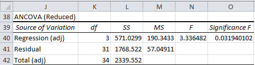
Figure 4 – Reduced ANCOVA model for Example 1
Here the adjusted regression SS (cell L40) is =L33 (from Figure 3), the residual SS (cell L41) is =L34, and the adjusted total SS (cell L42) is =L40+L41.
An alternative way of calculating SST in the reduced ANCOVA model uses the slope of the regression line that fits all the data points, namely (with reference to Figure 1 of Basic Concepts of ANCOVA)
bT = SLOPE(A4:A39,B4:B39) = 0.376975
![]()
Also note that SST(x,t) = DEVSQ(B4:B39).
Adjusted means
We now turn our attention to the treatment means
, including coefficients")
Figure 5 – Full model (y, x, t), including coefficients
Thus the regression model is
![]()
One thing this shows is that for every unit of increase in x (i.e. for every additional $1,000 of family income), y (i.e. the child’s reading score) tends to increase by .323 points.
Note that the mean value of x is given by AVERAGE(B4:B39) = 48.802 (using Figure 1).
To get the adjusted mean of the reading scores for Method 4, we set x = 48.802 and t1 = t2 = t3 = 0, and calculate the predicted value for y:
![]()
For Method 1 we set x = 48.802, t1 = 1 and t2 = t3 = 0.
![]()
Similarly, for Method 2 we set x = 48.802, t2 = 1 and t1 = t3 = 0.
![]()
Finally, for Method 3 we set x = 48.802, t3 = 1 and t1 = t2 = 0.
 Results
The results are summarized in Figure 6.

Figure 6 – Adjusted means for Example 1
The values for Y in Figure 6 are the group means of y. E.g. the mean of reading scores for Method 2 is AVERAGE(A12:A19) = 33.75. The adjusted grand mean is the mean of the adjusted means, i.e. AVERAGE(C56:C59) = 23.442.
The adjusted means can also be computed using the slope bW, which is the regression coefficient of x in the full model (i.e. the value in cell S36 of Figure 5), namely bW = .323.

Figure 7 – Alternative method for calculating the adjusted means
Here the values for Y are the group means as described above. The values for X (the covariate) are similar; e.g. the mean family income for the children in the Method 2 sample (cell C49) = AVERAGE(B12:B19) = 60.2625. The grand mean for the covariate (cell C52) is AVERAGE(B4:B39).
The adjusted means are now given by the formula
![]()
E.g. the adjusted mean for Method 2 (cell D49) is given by the formula =B49-S36*(C49-C52) where cell S36 contains the value of bW.
Examples Workbook
Click here to download the Excel workbook with the examples described on this webpage.
References
Howell, D. C. (2010) Statistical methods for psychology (7th ed.). Wadsworth, Cengage Learning.
https://labs.la.utexas.edu/gilden/files/2016/05/Statistics-Text.pdf
Schmuller, J. (2009) Statistical analysis with Excel for dummies. Wiley
https://www.oreilly.com/library/view/statistical-analysis-with/9780470454060/
How do I calculate the covariate, main, and interaction effects in 2-factor ANCOVA using regression? There is one covariate. I believe SSE can be calculated from the full model by regressing Y on x, I1, I2, I1I2. What about the other sum of errors?
Hello Vagela,
I have not yet supported 2-factor ANCOVA. I would imagine that the concepts that I have described on the following webpage would be applicable:
https://real-statistics.com/analysis-of-covariance-ancova/ancova-slopes-assumption-not-met/
Charles
Hi Charles,
thank you for these explanations.
I’m looking for an Excel-doable way to determine the p-value among intercepts and slopes, exactly how you explain in “Comparing slopes and intercepts” with the 2 t sper provided by the linear regression. However there we had only 2 groups. What if we have 3 or 4, like here? (especially if the number of datapoints aren’t constant between groups). The matrix architecture here looks like a natural scale-up of the concepts explained on the other page, but I’m still uncertain how to get the p values for “intercepts are all the same” and “slopes are all the same”. Are the significances in Figure 3 basically them? If not, do you have any resources where I can find a method for getting these 2 p values, or F values?
Thanks again.
Hello Lince,
I am sorry, but I need further clarification on your question. Are you asking me a question about the equal slope assumption for ANCOVA or something else?
Charles
Thank you.
Please, how the standard deviation of the fitted means can be calculated: ANCOVA. These means are necessary to calculate Cohen’s d with the adjusted means
Thanks
Dolores
Hello Dolores,
The following paper describes how to calculate the variance of the difference between two adjusted means. From these calculations you probably can figure out the variance of one adjusted mean.
http://www.glmj.org/archives/articles/Clason_v38n1.pdf
The following might also be useful>
https://ncss-wpengine.netdna-ssl.com/wp-content/themes/ncss/pdf/Procedures/NCSS/Analysis_of_Covariance-ANCOVA-with_Two_Groups.pdf
Charles
Hi, Charles
Thank you for your educational website operations.
I have learned ANCOVA on this website to teach my young colleague about ANCOVA.
I have a question about this article.
For Figure 3 – ANCOVA model for Example 1, why the sum of SS, Covariate, Treatment(adj.), and Residual, is not equal to Total SS?
Thank you,
Hiroshi
Hello Hiroshi,
The sum of the various SS values equals the SS Total for a balanced model ANOVA, but not necessarily for other models.
Charles
Hi, Charles
I’m doing experiment to looking for the effect of instruction media to time on task of a person in using a software. To make it as real as possible, I allow them to re-read the instruction based on their needs. Turns out that during the experiment, my respondents have various of frequency in re-read the instruction. Could the frequency of re-read the instruction become the covariate? if no, what should I do the reduce the bias?
Your answer will be much appreciated! Thankyou
Hello Salsa,
Sorry, but I don[t sufficiently understand the situation to be able to give a response.
Charles
You deserve thanks for your efforts.
Charles,
I have the following three comments for you:
1. The grand mean of the reading score presented in Figure 6 should be 23.05556.
2. I am not sure why the adjusted grand mean is the mean of the adjusted means when the sample sizes are not equal for individual methods.
3. There is an error on the formula for the adjusted means using the slop bw.
It should be y’j=yj – bw*(xj – xmean). The factors inside the parentheses were incorrectly listed.
-Sun
Hi Sun,
1. Yes, you are correct. This has now been corrected on the webpage.
2. This will give equal weight to each group even when the sizes are different.
3. Yes, you are correct. This has now been corrected on the webpage
Thanks once again for all your efforts to improve the website.
Charles
Hello, and thanks for all the effort on this blog. It is really a wealth of information.
I have a question regarding the suitability of co-variate.
I have three groups with different levels of production in pcs (low, medium, high), material waste in % and number of machine setup changes.
Can I use the number of machines setup changes as a co-variate, if in majority of cases high level of production is related to nigher number of machine changes?
I am almost certain that its not suitable as they are usually correlated (although it does not have to be the case), but needs external opinion and explanation.
If co-variate is not suitable, whats do you recommend me?
Thanks
Adriano,
If I understand your question correctly, then it simply depends on whether the assumptions for ANCOVA are met. Without seeing your data I can’t determine this.
Charles
Hi Charles,
a small inconsistency in one of your very useful examples above:
“From Figure 3, we see that the covariate is significant (p-value = 0.012 < .05), and so family income is significant in predicting reading scores."
The corresponding p-value in Figure 3 is 0.000006.
Stephan,
Thanks for catching this error. The value is probably left over from an earlier version of the example. I have now corrected the error on the webpage.
I really appreciate your help in improving the accuracy of the Real Statistics website.
Charles
Hi Dr. Zaiontz,
Thanks for all of the great work you have done putting this add-on together. Everything works great despite Excel’s “I don’t play well with others” attitude.
I have been struggling with choosing an appropriate method for analyzing a data set that I am working with. Initially I thought that simply using a step-wise linear regression, or even ANCOVA would suffice, but at this point I am not sure.
I am trying to determine which independent variables are truly significant in my model / that are affecting the dependent variable. I am not interested in constructing a predictive model (even though that may come out of this analysis) – I just want to know which independent variables affect my dependent variable. All of the reach measurements were derived through multiple reach tests with one person. 9 people went through reach tests (each in one location).
Dependent variable:
– reach
There is overlap and covariance between the independent variables.
Independent variables:
– left / right
– upper / lower
– perceived location difficulty (overlaps with left/right and upper/lower, contains groupings of specific locations)
*There are 3 perceived difficulty levels (0-2)
– specific location (overlaps with left/right, upper/lower, and perceived difficulty)
*There are 7 specific locations ie: left lower area 3, right upper area 1
– male / female
– weight (overlaps with weight and male/female)
– height (overlaps with weight and male/female)
– generation
Additional notes: generations, weight, and reach are not normally distributed (Shapiro Wilks Test): reach is normally distributed when segmented into specific locations ie: location 1 has normally distributed reach values as does location 2, but when binned together they do not (mean 1 != mean 2)
Height is normally distributed.
Thanks for any and all help. I’ve been chasing myself in circles for days now… in the industry that I am working in (medical) it is common to screen variables before putting them through a regression using a high p value (0.25) as a thresh hold. I don’t necessarily agree with the methodology but I should at least figure out how to appropriately do this per industry standards.
To further expand on this – the want of my higher ups is to limit the number of independent variables thrown into the multivariate regression by screening independent variables for covariance (with an alpha = 0.25) beforehand.
How to do so.. I’m not sure
Josh,
Here are several approaches, although these are not equivalent and so which one to choose depends on your specific requirement.
1. If you simply perform multiple regression you will see which variables have coefficients which are significantly different from zero. You could also use the Shapely-Owen Decomposition to see which variables are most important in the model.
2. If you use stepwise regression you will create a model all of whose variables are significant. It could still be that other variables are significant, but they don’t add anything to the stepwise model. E.g. if two variables are identical (or are highly correlated), then only one of these is necessary (or even desirable) in the stepwise regression model, but the other could be used instead of the first.
3. You could do one linear regression for each independent variable to see whether that variable has a significant regression coefficient.
Charles
From what I can tell the step-wise linear regression seems the most appropriate. That being said, is there a way to see which variables are significant but are not included in the step-wise model due to high correlation with another variable?
For example: left/right and upper lower vs perceived location difficulty with inevitably be highly correlated (or at least I would expect them to be). I could just do a step-wise linear regression with only one location based variable included each time.. but is there a more official way to initially test and ascertain for high correlation/covariance? Conversely, what is most important to test for, correlation or covariance?
Thanks again, your responses are much appreciated.
Josh,
1. You can use Excel’s Correlation data analysis tool to generate all pairwise correlations between the variables. This will tell you which variables are highly correlated with one other. This does not tell you which may be highly correlated with a combination of other variables. You could do separate multiple regressions to determine this, although this is a lot of work.
2. Alternatively you could use the Real Statistics CORR array function to generate all pairwise correlations. You can also use the Real Statistics RSquare function to determine the correlation between one variable and any number of other variables.
3. The stepwise regression option to the Real Statistics Multiple Regression data analysis tool will show you how the regression variables are being chosen in the stepwise model.
4. Correlation is easier to interpret than covariance, since near 1 or near -1 indicates high correlation.
Charles
Your responses have been crucial to my understanding of this problem but have also sparked more questions!
1. I did as you suggested and used Excel’s Correlation tool – I now have a matrix of Pearson’s coefficients. Does the Excel tool appropriately treat differing units/unit types? I had read a bit into the usage of Spearman’s Rank Correlation as a means of avoiding the shortfalls of a “normal” correlation test.
2. When testing the significance of the Pearson coefficients in the matrix, I was surprised by the number of variables that were significant at alpha = 0.05. I assume that this is due to the large sample size (n = 184). This in turn leads me to believe that using n = 184 is not necessarily appropriate.
3. In thinking of ways to account for this, I decided to focus on the actual question at hand and boiled it down to one of two questions (which I think are synonymous).
a.) Is Region (upper/lower) correlated to perceived difficulty.
b.) Are the reach values for given regions (upper/lower) correlated to the reach values for perceived difficulty tiers.
While the question posed under b.) is a bit more convoluted it gets around one concern I had for question a.): Can you compare dichotomous data, ordinal data, AND categorical data in a correlation test? – I know that categorical doesn’t fit in completely but I assigned #1-20 for the 20 different specific locations (categories)
As an example: Column A: 1,1,1,0,0,0,1,1,1 (dichotomous based off of designation as upper or lower); Column B: 2,2,2,0,0,0,1,1,1 (ordinal based off of perceived difficulty); Column C: Category1, cat1, cat1, cat2, cat2, cat2, cat3, cat3, cat3 (categorical based off of specific location)
I felt uneasy just throwing those three columns into Excel’s Correlation test, hence my proposed solution in question b.).
While b.) purely deals with continuous data, the sample size of each varies. ie: there are 11 samples done for upper, 15 for lower vs 8 for difficulty 0, 7 for 1, and 11 for 2… and so on and so on.
Lastly: is there a certain point where you just say that enough is enough and assume correlation based off of known facts? Perceived difficulty is a made up variable based off of our observations and is DIRECTLY pulled from the specific location. Values in locations 1-4 (upper) are the most difficult, 5-6 (lower) are medium, and 7-10 are easy.
Sorry for the whale of a question…
Josh,
1. I don’t quite know what you mean by “differing units/unit types”. Correlation is units-free. In any case, Excel uses its CORREL function (or an equivalent) to calculate the values in the table. If you prefer to create a similar table, you can first calculate the ranks of all the data elements (using RANK.AVG) and then use the Correlation data analysis tool on this data.
2. There is nothing wrong with using a large sample size, but you have noticed something important, namely that the bigger the sample size the more likely you will find a significant result. Note that “significant” is not the same as “large”. Also remember that significant for correlation probably means significantly different from zero.
3. Let me make a few observations, which may not directly answer your question, but may help you find the answer.
(a) You can certainly calculate the correlation between dichotomous variables or dichotomous and continuous variables. This is commonly done. The latter is called point-biserial correlation (but it is equivalent to Pearson’s correlation).
(b) Correlation analysis between a categorical variable and a continuous variable is really equivalent to a t test or ANOVA, as described on the following webpages:
https://real-statistics.com/correlation/dichotomous-variables-t-test/
https://real-statistics.com/multiple-regression/anova-using-regression/
Charles
Dear Professor
Thanks for your page so much.
I have issue that need your help. I want to test the parallel between 2 linear regression- line. Firstly, i test the linear regression of two model. Then i want to test the parallel of these two. I think i can use the comparision of slopes of each model. if there ‘s no significantl difference between these two, they are parallel with each other. Is my method right or wrong?
I hope you can answer me.
thanks and best regards.
Yes, this is correct.
Charles
Hi professor,
thank you for this page, it is really helpful! I am a not sure about some definitions and I would like to know what is the difference between adjusted, balanced and weighted in statistics ?
thank you very much!
Stephanie
Stephanie,
The meanings of these terms depend on the context in which they are used. In the case of ANCOVA, adjusted implies that we make some change to the normal definition for some specific purpose. Balanced generally means that multiple groups have the same number of elements. Weighted means that you multiply each k-tuple of values by a fixed k-tuple of weights.
Charles
Thank you very much for all your work!
What I don’t understand is:
To get the adjusted means we count “mean_1 – (b_x *(mean_x1 – mean_x)” where mean_1 is the mean of group1, mean_x1 is the mean of the covariate over group1, mean_x is the mean of the covariate over all subjects and b_x is the weight of the covariate.
How can I get b_x without knowing the adjusted means? When I do a regression of x on y, I don’t get the same b_x as in the full model. thanks!
Mik,
As stated at the bottom of the referenced webpage, b_W is equal to the b_x (cell S36 in Figure 5). This is what we need to calculate the adjusted means. You can also calculate b_W and the adjusted means using the ANOVA approach, as described on the webpage ANCOVA using ANOVA.
The value b_x is calculated using the regression shown in Figure 5 without adjusting the means.
Charles
Dr. Zaiontz
First I would like to thank you remarkable effort for bringing such a creative tutorial type statistics website.
I am writing to seek your advice on some data analysis.
We are trying to evaluate relative potency of drug and want to compare with some reference drug.
Design of experiment is as below
1) Both Test and reference drug is tested in parallel with reference drug at five doses @ 1/3 log variation in animals
2) for each dose, we are having a group comprise of 10 animals so in total 50 animals each for test and reference totalling 100 animals
3) After drug injection, potency in animals are checked through certain assay which gives quantitative values.
Now question are
1) which of statistical method is good way to judge and conclude Test drug is having same potency that of reference drug. whether we should use Anova or ANcova or something else for analysis?
2) Which statistical test is right way to evaluate its significance? F test or T test
Thanks in anticipation
Based on my understanding of the scenario, you have two factors: Factor A has two levels test and reference drug. Factor B has 5 levels for the 5 dosages. This is a classic two fixed factor ANOVA, which uses an F test. When you get into follow up analyses, you may use a t test.
Charles
Sir,
I have four covariates with three factors/treatments, can you explain how to calculate ANCOVA with this several covariates? and can i know what the best treatments in this case?
Thank You,
Citra
Citra,
Sorry, but I have not dealt with the case of multiple covariate as of yet. I will eventually add this. I believe that SPSS handles this type of analysis.
Charles
Hello,
Thanks for your page and your practice sheets. I was trying this out with my analysis where I only have 2 treatment groups (instead of 4 like yours). I was finding that when I run the linear regressions, it would return “0” for coefficient, standard deviation, and upper/lower limits for…
-“x” and “t1” in the complete regression
-“t1” for the full regression
-“t1” for the y,t partial
-“t1” for the x,t partial
As far as I can see I’m setting up my tables exactly the same as you, would you have any thoughts what I may be doing wrong?
Charity
Sir,
Would you please be so kind and explain, how the intercept (in the above ex. 2,857) is calculated in ANCOVA
Franz,
The full model (including the intercept) is obtained using ordinary linear regression on the data in Figure 1. This is done by running either Excel’s Regression data analysis tool or the Real Statistics Linear Regression data analysis tool (see webpage https://real-statistics.com/multiple-regression/ for details)
Charles