Positive and null recurrence

Basic Concepts

Suppose i is a recurrent state (see Connectivity). i is positive recurrent if n_i < ∞ and null recurrent if n_i = ∞ (see Hitting Probabilities for the definition of n_i).

Property 1:  In a recurrent class, all states are positive recurrent or all states are null recurrent.

Proof: The proof is similar to that of Property 4 of Connectivity.

Property 2: In a finite closed class, all states are positive recurrent.

Proof: The proof is similar to that of Property 7 of Connectivity.

Based on these properties and related properties in Connectivity, we observe that

• Non-closed classes are transient
• Closed classes in finite Markov chains are positive recurrent
• Closed classes in infinite Markov chains can be transient, null recurrent or positive recurrent.

As we observe in Connectivity, for a one-dimensional random walk with p ≠ .5, all states are transient. When p = .5 all states are recurrent, but as we observe in Random Walks, n₀ = ∞, and so all states are null recurrent.

Existence/uniqueness of a stationary distribution

Property 3: For an irreducible Markov chain

• If the chain is positive recurrent, then a unique stationary distribution π exists where π_i  = 1/n_i, where n_i is the expected time to return to state i.
• If the chain is null recurrent or transient, then no stationary distribution exists

Even if the Markov chain is not irreducible, Property 3 applies to any communications class that is positive recurrent (and so is closed). The unique stationary distribution applies only to that class.

By Property 7 of Connectivity, a finite, irreducible Markov chain is always positive recurrent, and so Property 3 holds.

Stationary distribution example

Example 1: Find the stationary distribution for the transition matrix in range B2:D4 of Figure 1.

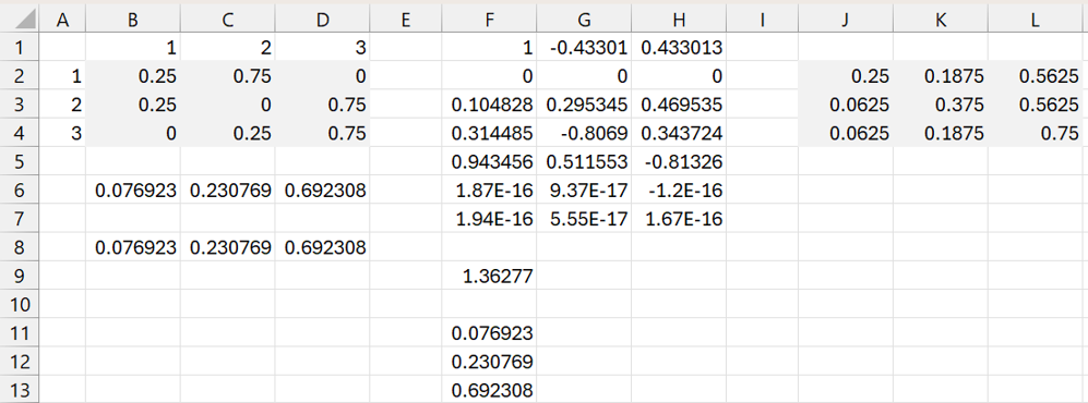
Figure 1 – Stationary distribution

First note that the formula =MPOWER(B2:D4,2) yields the matrix in range J2:L4. Since all the elements in this matrix are positive, per Property 4 of Markov Chain Distributions, there is a unique stationary distribution. This distribution is displayed in range B6:D6, using the approach described in Markov Chain Distributions. We see that the formula =MMULT(B6:D6,B2:D4) yields the results shown in range B8:D8, namely (1/13, 3/13, 9/13),

We note that 1 ↔ 2 ↔ 3, and so the chain is irreducible. Since the Markov chain is finite and there is one communications class, by Property 7 of Connectivity, it is recurrent, and so t_i = 1 for i = 1, 2, 3.

We can calculate n₁₁, n₂₂, and n₃₃, as described in Hitting Probabilities.

Calculating n₁₁

k₃₁ = 1 + .25 k₂₁ + .75 k₃₁

.25 k₃₁ = 1 + .25 k₂₁

k₃₁ = 4 + k₂₁

k₂₁ = 1 + .25 k₁₁ + .75 k₃₁ = 1 + .25(0)+ .75(4+k₂₁)

.25 k₂₁ = 1 + 3

k₂₁ = 4(4) = 16

n₁₁ = 1 + .25 k₁₁ + .75 k₂₁ = 1 + .25(0)+ .75(16) = 13

Calculating n₂₂

k₁₂ = 1 + .25 k₁₂ + .75 k₂₂

.75 k₁₂ = 1 + .75(0)

k₁₂ = 4/3

k₃₂ = 1 + .25 k₂₂ + .75 k₃₂

.25 k₃₂ = 1 + .25 k₂₂ = 1 + .25(0) = 1

k₃₂ = 4(1) = 4

n₂₂ = 1 + .25 k₁₂ + .75 k₃₂ = 1 + .25(4/3) + .75(4) = 1 + 1/3 +3 = 13/3 = 4.3333

Calculating n₃₃

k₁₃ = 1 + .25 k₁₃ + .75 k₂₃

.75 k₁₃ = 1 + .75 k₂₃

k₁₃ = 4/3 + k₂₃

k₂₃ = 1 + .25 k₁₃ + .75 k₃₃ = 1 + .25 k₁₃ + .75(0)

= 1 + .25(4/3 + k₂₃)

.75 k₂₃ = 1 + .25(4/3) = 4/3

k₂₃ = (4/3)(4/3) = 16/9

n₃₃ = 1 + .25 k₂₃ + .75 k₃₃ = 1 + .25(16/9) + .75(0) = 1 + 4/9 = 13/9 = 1.4444

Using Property 3

Since this Markov chain is finite, by Property 2, all the states are positive recurrent, and so Property 3 holds.

Clearly, it is much easier to use Property 3 to calculate n₁₁, n₂₂, and n₃₃.

Multiple stationary distributions example

Example 2: Find the stationary distributions for the transition matrix in range B2:E5 of Figure 2.

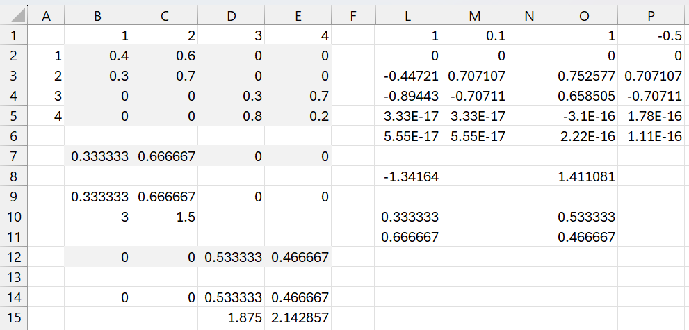
Figure 2 – Two closed classes example

For this example, we see that we have two closed classe {1, 2} and {3, 4}. We can use the eigVECT function on  each of the classes (as shown on the right side of the figure) to obtain the distribution shown in range B7:E7 for the first closed class, and the distribution shown in range F8:G9 for the second closed class.

Next, we confirm that each of these is a stationary distribution, using the formulas =MMULT(B7:E7,B2:E5) and =MMULT(B12:E12,B2:E5), as shown in ranges B9:E9 and B14:E14, respectively.

We can also obtain the values n₁₁ = 3 and n₂₂ = 3/2 = 1.5 from the reciprocals of the values in B7 and C7. Similarly, we obtain the values n₃₃ = 15/8 = 1.875 and n₄₄ = 15/7 = 2.142857 from the reciprocals of the values in D12 and E12.

Example with a transient class

Example 3: Find the stationary distribution for the transition matrix in range B2:E5 of Figure 3.

This Markov chain has one transient class  {1, 2} and one (positive) recurrent class  {3, 4}.  Using eigVECT, we see that (0, 0, 8/15, 7/15) is a stationary distribution, as shown B12:F12.

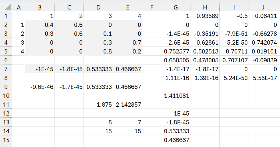
Figure 3 – One transient and one recurrent class

n₁₁ = n₂₂ = ∞ for the transient class, and n₃₃ = 1/.53333 = 1.875 = 15/8 and n₄₄ = 1/.4667 = 2.142857 = 15/7 for the recurrent class.

Examples Workbook

Click here to download the Excel workbook with the examples described on this webpage.

Links

↑ Markov chains

References

Aldridge, M. (2021) Recurrence and transience. Introduction to Markov Processes
https://mpaldridge.github.io/math2750/S09-recurrence-transience.html

Norris, J. (2004) Discrete-time Markov chains. Cambridge University Press
https://www.statslab.cam.ac.uk/~jrn10//Markov/