Stationary distributions
Associated with a Markov chain is a probability distribution πi for each xi.
If the set of states is S = {1, …, n}, then the probability distribution for xi is an n × 1 row vector whose jth element is P(xi = j). If P is the transition matrix for a Markov chain and π is a probability distribution for x0, then the corresponding probability distribution πi for xi is
πi = πPi
A distribution π is stationary (aka invariant) if
π = πP
In this case, for any n > 0
π = πPn
Perron-Frobenius Theorem
We now take a short detour and speak about square matrices in general, before returning to the case where the square matrix is a transition matrix of a Markov chain. We reference eigenvalues and eigenvectors. See Eigenvalues and Eigenvectors for more details.
A matrix A is non-negative if all its elements are non-negative.
An n × n matrix A is irreducible if for all i, j ≤ n, there is a k such that the element (i, j) in Ak is positive. Different i, j may require different values of k.
An n × n matrix A is primitive if there is a k such that all elements in Ak are strictly positive
Property 1 (Perron-Frobenius Theorem): If A is a non-negative square matrix whose dominant eigenvalue is λ*, then
- λ* is real-valued and non-negative
- λ* has a corresponding non-negative eigenvector
If A is irreducible, then
- λ* has a corresponding strictly positive eigenvector
- there are no other strictly positive eigenvectors associated with λ*, except scalar multipliers
If A is primitive, then
- λ* > |λ| for any other eigenvalue λ
Applications to Markov Chains
We now return to the subject of Markov chains, and shortly we explain how to apply the Perron-Frobenius Theorem to Markov chains.
Property 2: The dominant eigenvalue of a transition matrix is 1.
Proof: Let P = an n × n transition matrix, and define λ = 1 and X = the column vector consisting of n 1’s. Since all the rows in P sum to 1, the following is true
PX = X = λX
This proves that X is an eigenvector associated with the eigenvalue 1.
Now, suppose that P has an eigenvalue λ where |λ| > 1. Then, for all n, PnX= λnX. Thus, λ2n→ ∞ as n → ∞, which means that for n large enough, P2n contains some element larger than 1, which is a contradiction since powers of P can only contain elements between 0 and 1.
Note that an eigenvalue of a square matrix A is also an eigenvalue of its transpose. This follows since if det(A–λI) = 0, then det(AT–λI) = det(A–λI) = 0.
Property 3: Every Markov chain has at least one stationary distribution.
Proof: This is the transpose of the eigenvector of PT corresponding to the dominant eigenvalue with value 1 (per Property 2). By the Perron-Frobenius Theorem this eigenvector has non-negative elements, which is sufficient to prove the property since you can always find a scalar multiplier such that the eigenvector is a distribution vector (e.g. see Example 1 below).
Property 4: If the transition matrix P (or Pn for some n) only has positive entries, then there is only one stationary distribution.
Proof: This follows from the Perron-Frobenius Theorem.
Multiple stationary distributions
When the eigenvalue 1 is repeated, the Markov chain has multiple stationary distributions, one for each eigenvalue of 1. In fact, in this case, any linear combination of the eigenvectors associated with these eignevalues is also an eigenvector associated with eigenvalue 1. Thus, there are an infinite number of stationary distributions. In particular, if the coefficients are positive and sum to one, then the linear combination is also a stationary distribution. See Example 1.
Examples
Find the invariant/stationary distributions for the Markov chains with the transition matrix P shown in range A1:C3 (whose transpose is shown in A5:C7).
Example 1
We use the Real Statistics formula =eigVECT(A5:C7) to calculate the eigenvalues/vectors for PT. We see that two of the eigenvalues are 1, with a third whose value is less than 1. The eigenvectors associated with eigenvalue 1 are shown in ranges E3:E5 and F3:F5. Note that the elements in each vector are non-negative.
These are unit eigenvectors, and so the sum of the squares of the elements in each is one. Since we are looking for a probability distribution, we want eigenvectors whose elements sum to one. These are shown in ranges E11:E13 and F11:F13. We obtain the first of these by summing the values in the first eigenvector, as shown in cell E9, using the formula =SUM(E3:E5). We then divide each element in E3:E5 by the sum 1.264034 to obtain the desired vector; e.g. cell E11 contains the formula =E3/E$9.
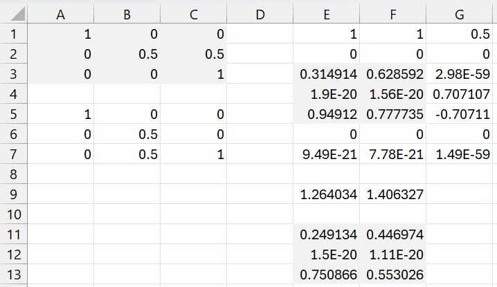
Figure 1 – Two invariant distributions
We repeat this procedure to obtain the distribution vector shown in range F11:F13. Actually, the distribution vectors are the transposes of these, namely (.249134, 0, .750866) and (.446974, 0, .553026). In fact, =MMULT(TRANSPOSE(E11:E13),A1:C3) outputs the row vector (.249134, 0, .75066), as expected, and similarly for the second distribution vector.
As noted above, since (.249134, 0, .750866) and (.446974, 0, .553026) are stationary distributions so is any linear combination whose coefficients are non-negative and sum to one. For example the following is also a stationary distribution.
.4(.249134, 0, .750866) + .6(.446974, 0, .553026) = (.367838, 0, .632182)
Example 2
We repeat the same procedure to calculate a distribution vector for the transition matrix in range A1:C3 of Figure 2, namely (.356322, .264368, .37931).
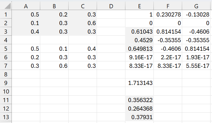
Figure 2 – Unique distribution vector
We note that – this time – all entries in the transition matrix are positive. As expected, there is a unique distribution vector. Also, note that the one eigenvalue is not repeated, and the absolute values of the other eigenvalues are less than 1.
Example 3
We repeat the same procedure to calculate a distribution vector for the transition matrix in range A1:C3 of Figure 3, namely (1/3, 1/3, 1/3).
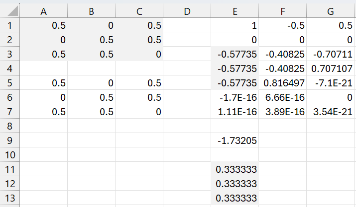
Figure 3 – Non-positive transition matrix
Although the transition matrix contains zero values, there is a unique distribution vector. Note, however, that =MPOWER(A1,C3,2) produces an array with only positive values. For Example 1, however, Pk contains zero elements for any value of k.
Examples Workbook
Click here to download the Excel workbook with the examples described on this webpage.
Links
References
Konstantopoulos, T. (2009) Markov chains and random walks
https://www2.math.uu.se/~takis/L/McRw/mcrw.pdf
Knill, O. (2011) Linear algebra with probability
https://people.math.harvard.edu/~knill/teaching/math19/math19b_2011.pdf