Basic Concepts
In a sample taken from a population, the kth order statistic is the kth smallest element in the sample. We describe the distribution of the kth order statistic when a sample of size n is randomly drawn from the population {1, 2, …, N} (without replacement).
In particular, we see that the probability density function is
![]()
for integer values of x, 1 ≤ x ≤ N, and f(x) = 0 otherwise.
The probability density function of the joint probability distribution of the smallest and largest elements in a random sample of size n > 1 drawn from the population {1, 2, …, N} is
![]()
for integer values of x and y where, 1 ≤ x ≤ y ≤ N, and f(x, y) = 0 otherwise.
Example 1
Suppose that you draw a sample of size 10 from the population {1, 2, …, 25}. (a) What is the probability that the smallest element in the sample is 3? (b) What is the mean value of the smallest element in the sample? (c) What is the probability that the smallest and largest elements in the sample are 1 and 25?
The probability that 3 is the smallest element in the sample (part a) is .152174, as shown in cell B10 of Figure 1.
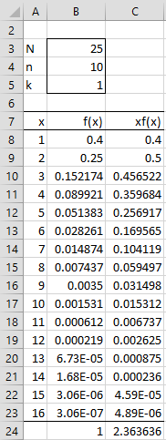
Figure 1 – Order statistics
Cell B10 contains the formula
=COMBIN(A10-1,B$5-1)*COMBIN(B$3-A10,B$4-B$5)/COMBIN(B$3,B$4)
To find the mean of the smallest values (part b), we calculate the probabilities (column B) of each possible outcome for the smallest value. These are the x values from 1 to N-n+1 = 25-10+1 = 16 in column A. We next multiply these probabilities by the x value (column C); the sum of these values is the mean. We see from cell C24 that the mean is 2.3636.
We can calculate the probability that the smallest and largest values in the sample are 1 and 25 respectively (part c) by the formula =COMBIN(H8-G8-1,B4-2)/COMBIN(B3,B4), which has the value 0.15.
Example 2
Suppose that you draw a sample of size 5 from the population {1, 2, …, 10}. (a) What is the mean value of the range in the sample (i.e. the difference between the largest and smallest values)? (b) What is the probability that the range in the sample is 5?
For Part (a) we proceed in a manner similar to that for Example 1, as shown on the left side of Figure 2.

Figure 2 – Range statistics
In Figure 2, the possible pairs of smallest and largest values are shown in columns A and B. Column C now contains the probabilities f(x,y) that x is the smallest value and y is the largest value. E.g. the probability that 1 is the smallest value and 5 is the largest value in the sample is 0.003968, as shown in cell C7 using the formula =COMBIN(B7-A7-1,B$4-2)/COMBIN(B$3,B$4).
The mean value is computed as for Example 1 using the range values in column D. E.g. cell E7 contains the formula =D7*C7 and cell E28 contains the formula =SUM(E7:E27). The mean is 7.333, as shown in cell E28, thus completing Part (a).
Note that to obtain the values in columns A and B, we insert 1 and 5 in cells A7 and B7. Then we place the formula =IF(B7<B$3,A7,A7+1) in cell A8 and the formula =IF(B7<B$3,B7+1,A8+B$4-1) in cell B8. By highlighting the range A8:B7 and pressing Ctrl-D, we fill in the remaining values in columns A and B.
For Part (b), the probability that 5 is the difference between the largest and smallest value in the sample is .0793665. This result is obtained in cell J8 by using the formula =SUMIF(D$7:D$27,I8,C$7:C$27).
Calculating C(n,m) for large values of n and m
For relatively small values of N and n, the approach described in Example 1 and 2 using the COMBIN function works quite well. For larger values of N and n, COMBIN yields an overflow message. E.g. =COMBIN(1200,338) takes the value 1.8+E308, but =COMBIN(1200,338) takes the value #NUM!
Since the values that we are interested in are probabilities that take values between 0 and 1, we can avoid the overflow problem by using the natural logarithm of C(n, m) instead of C(n, m). In particular
![]()
which in Excel can be calculated as
=GAMMALN(n+1) + GAMMALN(m+1) – GAMMALN(n-m+1)
As described below, Real Statistics provides the function LNCOMBIN(n, m) which takes the value ln C(n, m) as calculated using the above formula.
Using the above trick, the probability that x is the kth order statistic can be calculated in Excel by the formula
=EXP(LNCOMBIN(x–1, k–1) + LNCOMBIN(N–x, n–k) – LNCOMBIN(N, n))
where you can use the Real Statistics function LNCOMBIN or substitute formulas involving GAMMALN as described above. This approach is valid even for large values of N and n.
Worksheet Functions
Examples 1 and 2 can be addressed by the following Real Statistics functions.
Real Statistics Functions: The Real Statistics Resource Pack supplies the following functions:
ORDERDIST(x, N, n, k) = the probability that x is the kth order statistic when a random sample of size n is drawn from {1, 2, …, N}; if k is omitted it defaults to 1.
MEANORDER(N, n, k) = the mean value of the kth order statistic when a random sample of size n is drawn from {1, 2, …, N}; if k is omitted it defaults to 1.
RANGEDIST(x, y, N, n) = the probability that x and y are the smallest and largest elements in a random sample of size n drawn from {1, 2, …, N)
MEANRANGE(N, n) = the mean value of the difference between the largest and smallest elements in a random sample of size n drawn from {1, 2, …, N)
SPANDIST (x, N, n) = the probability that x is the difference between the largest and smallest elements in a random sample of size n drawn from {1, 2, …, N}.
LNCOMBIN(x, y) = natural log of C(x, y)
We can obtain the results for Examples 1 (a), (b), (c) by using the worksheet formulas =ORDERDIST(A9,B3,B4,B5), =MEANORDER(B3,B4,B5), =RANGEDIST(1,25,B3,B4), respectively.
We can obtain the results for Examples 2 (a) and (b) by using the worksheet formulas =MEANRANGE(B3,B4) and =SPANDIST(5,B3,B4).
Examples Workbook
Click here to download the Excel workbook with the examples described on this webpage.
Reference
Evans, D. L., Leemis, L. M., Drew, J. H. (2006) The distribution of order statistics for discrete random variables with applications to bootstrapping. INFORMS Journal on Computing Vol. 18, No. 1, pp. 19–30.
https://www.rose-hulman.edu/~evans/pdf/JOC_OrderStat.pdf