We now describe the distribution of order statistics from a continuous uniform population. To keep things simple, we consider the population on the unit interval (0, 1).
First, let’s look at the general case where the population has a continuous distribution with pdf g(y) and cdf G(y). We start by describing the (cumulative) distribution F(x) of the kth order statistic in a sample of size n taken from the population.
Properties
Property 1: The cdf of the kth order statistic is
![]()
Proof:
F(x) = the probability that the kth order statistics is less than or equal to x
= P(at least k elements in the sample are less than or equal to x)
![]()
The result now follows since we have a binomial distribution.
Property 2: The pdf of the kth order statistic is
![]()
Proof: This is Property 3 of Order Statistics from a Continuous Distribution. The proof is described in Order Statistics Proofs.
Property 3: If the population follows the uniform distribution on the interval (0,1), the kth order statistic has a beta distribution Bet(k, n-k+1).
Proof: If the population distribution is the uniform distribution on the interval (0,1) then g(x) =1 and G(x) = x. By Property 2
![]()
![]()
But, this last term is the pdf for the beta distribution Bet(k, n-k+1), thus completing the proof.
Property 4: If the population follows the uniform distribution on the interval (0,1), the mean and variance of the kth order statistic are
![]()
Proof: By Property 3 and the formulas for the mean and variance of the beta distribution, we have![]()
![]()
Area under the Curve
Let’s consider the area under the curve y = G(x) between x = 0 and x = 1. Then the area under the curve between x = μk and x = μk+1 is
![]()
The area under the curve from x = 0 to x = μ1 is also 1/(n+1), as is the area under the curve from x = μn to x = 1.
![]()
Thus, the lines x = μk divide the area under the curve y = G(x) into n+1 regions each with area 1/(n+1). Now, for any given sample of size n, if the order statistics are xk, then for any k, we have E[xk] = μk, and so E[G(xk)] = G(μk) = k/(n+1). Thus E[G(xk+1)–G(xk)] = 1/(n+1), and similarly E[G(x1)–0] = 1/(n+1) and E[1–G(xn)] = 1/(n+1).
Therefore, on average, the order statistics in a sample tend to divide the area under the curve y = F(x) into n+1 regions, each with area 1/(n+1).
It now follows that the order statistics can be used as estimates of the percentiles of a distribution. In fact, this is how the percentiles were calculated, using PERCENTILE.EXC, in Ranking Functions in Excel.
Median Example
Example 1: Estimate the population median based on the sample shown in range B3:F9 of Figure 1. Also, estimate the 95% confidence interval for the population median.
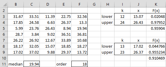
Figure 1 – Confidence Interval for the Median
Using the formula =MEDIAN(B3:F9) we see that 19.94 is the median of the sample. We can use this value as an estimate for the population median. This value is the 18th order statistic x18 in the sample, where 18 is calculated by the formula =INT((COUNT(B3:F9)+1)/2).
Confidence Interval
We now determine how likely it is that the population median m is actually in the interval (x15, x21). Using a bit of trial and error, we chose the order statistics 6 units away from the median on either side. For any element in the population chosen at random, the probability that this element is less than the median is p = .5.
The probability that m is in the interval (x12, x24) is equal to the probability that at least 12 elements in the sample are less than m and less than 24 elements in the sample are less than m. This probability is
![]()
As we can see from the right side of Figure 1, (x12, x24) is the interval (15.07, 26,43), which represents a 95% confidence interval. Alternatively, this probability is equal to F(x24-1) – F(x12-1) where F(x) is the cdf for the binomial distribution B(35,.5). This can be calculated in Excel by the formula
=BINOM.DIST(11,35,.5,TRUE)-BINOM.DIST(23,35,.5,TRUE)
.9% confidence interval. Here, 15.07 and 26.43 are calculated by the formulas =SMALL($B$3:$F$9,I3) and =SMALL($B$3:$F$9,I4) in cells J3 and J4. Cell K3 contains the formula =BINOM.DIST(I3-1,COUNT($B$3:$F$9),0.5,TRUE), cell K4 contains the formula =BINOM.DIST(I4-1,COUNT($B$3:$F$9),0.5,TRUE) and cell K5 contains the formula =K4-K3, resulting in the size of the confidence interval, namely .959.
If we decrease the size of the confidence interval by one order on each side, we see in cell K10 that (x12, x24) is a 91% confidence interval, farther away from 95% than (15.07, 26.43). This process is unlikely to arrive at a confidence interval that is exactly our objective of 95%, but it will yield a useful confidence interval. We could interpolate between the 95.9% and 91.0% confidence intervals, but we won’t pursue this further here.
Quartile Example
Example 2: Estimate the 3rd population quartile and the 95% confidence interval based on the sample from Example 1.
We use the same approach as for Example 1, except that this time we estimate the 3rd population quartile by the 3rd sample quartile, which is 29.37 (cell C16 in Figure 2) as calculated in Excel by the formula =QUARTILE.EXC(B3:F9,3). The 3rd quartile is the same as the 75th percentile (3/4 = 75%), and so 29.37 is the 27th order statistic where 27 in cell F16 is calculated by the formula =INT((COUNT(B3:F9)+1)*0.75).
This time we try the interval (x22, x32), whose endpoints are 5 orders from x27. Using the same approach as for Example 1, this is the interval (26.22, 33.89). We can calculate that this is slightly bigger than a 95% confidence interval (cell K18) by again using the binomial distribution, this time with p = .75 instead of .5.
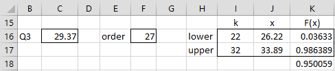
Figure 2 – Confidence interval for Q3
By moving the endpoints 2 more orders to the left and right (i.e. by changing cells I16 and I17 to 20 and 34, we can see that (23.76, 36.81) is a 99.3% confidence interval. To obtain a 99.9% confidence interval, we need to move the endpoints yet another 2 orders to the left and right. The only problem this time is that would require using the 36th order statistic on the right end, which is impossible since the sample size is only 35. Thus, we will use the interval (x18, x35) instead. This results in the 99.93% confidence interval (19.94, 37.02).
Observation
Note that we can use the beta distribution to provide estimates for the order statistics for the discrete uniform distribution, as described in Order Statistics from Finite Population. In particular, let’s re-examine Example 1(b) from Order Statistics from Finite Population. The mean value of the 1st order statistic for a sample of size 10 from a uniform distribution on the interval (0,1) is k/(n+1) = 1/11.
Since we need to map the interval (0,1) onto the interval (1, N), we need to multiply 1/11 by N+1 = 26 to obtain (1/11)(26) = 2.3636, which matches the result we obtained previously.
In general, the mean of the kth order statistic for a sample of size n taken from the discrete population {1, …, N} is
![]()
The situation is similar for the variance, namely
![]()
Examples Workbook
Click here to download the Excel workbook with the examples described on this webpage.
References
Border, K. C. (2016) Lecture 15: Order statistics; conditional expectation. Caltech
https://healy.econ.ohio-state.edu/kcb/Ma103/Notes/Lecture15.pdf
Ma D. (2010) The distribution of the order statistics. A Blog on probability and statistics
https://probabilityandstats.wordpress.com/2010/02/20/the-distributions-of-the-order-statistics/
Ma, D. (2010) Confidence intervals for percentiles. A Blog on probability and statistics
https://probabilityandstats.wordpress.com/2010/02/22/confidence-intervals-for-percentiles/
Ma, D. (2010) The order statistics and the uniform distribution. A Blog on probability and statistics
https://probabilityandstats.wordpress.com/2010/02/21/the-order-statistics-and-the-uniform-distribution/