Survivability and the Weibull Distribution

Basic Concepts

A survival curve can be created based on a Weibull distribution. We show how this is done in Figure 1 by comparing the survival function of two components: Part 1 with an alpha parameter of 1,120 and beta parameter of 2.2, and Part 2 with alpha = 1,080 and beta = 2.9.

E.g. cell B8 contains the formula =1-WEIBULL($A8,2.2,1120,TRUE), and similarly for the other cells. The chart is created by highlighting range B6:C27 and selecting Insert > Chart|Line Chart and making modifications as described in Line Charts.

As you can see, initially a Part 2 component is more likely to survive, but at about x = 1,000 (actually closer to x = 964), the situation changes and Part 1 components are more likely to survive longer.

Figure 1 – Survival plots for Weibull distribution

Survival Times

We can also ask at what time is a given level of survivability achieved. This is shown in Figure 2.

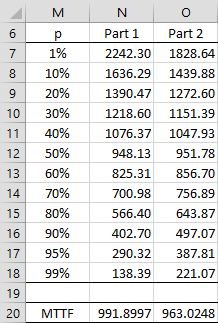
Figure 2 – Survival times

E.g. 60% of the Part 1 components are still functioning at time 825.31 (cell N13) as calculated by the formula =WEIBULL_INV(1-$M13,2.2,1120). The mean time to failure (MTTF) is also the mean survival time and is calculated as shown in Figure 1 of Weibull Distribution. For Part 1 this 991.9 as calculated by the worksheet formula =B3*EXP(GAMMALN(1+1/2.2)).

Examples

Example 1: Suppose a Part 1 component, as described above, survives to time 800, what is the probability that it will survive to at least time 1,600?

Let E = the event of survival until time 800 and F = the event of survival to at least 1,600. We seek the conditional probability P(F|E). As described in Basic Probability Concepts, P(F|E) = P(E∩F)/P(E) = P(F)/P(E), which can be calculated by the formula =B23/B15 (referring to Figure 1). Thus the answer is .111725/.620643 = 18%.

Example 2: Suppose a Part 1 component, as described above, survives to time 800, what is the median additional life span of the component?

Let E = the event of survival until time 800 and H = the event that the component survives to at most the median additional life span. As we saw in Example 1, P(H|E) = P(E∩H)/P(E) = P(H)/P(E) = .5, where .5 represent the median. Thus, P(H) = P(E)*.5 = .620643/2 = .31032. The event that the component survives to at least the median additional life span is 1 – P(H) = .68968. Using the inverse function, we get WEIBULL_INV(.68968,2.2,1120) = 1202.92. Thus, the median additional life span is 1202.92 – 800 = 402.92.

Example 3: Repeat Example 2 using the 80th percentile instead of the median.

P(H) = P(E)*.8 = .620643*(1-.8) = .124129. WEIBULL_INV(1-.124129,2.2,1120) = 1564.596. The result is 1564.596 – 800 = 764.596.

Mean Residual Life

Suppose a component has survived at time t, then the mean residual life, MRL(t), of this component is the conditional MTTF given that the component has survived until time t. Note that MRL(0) = MTTF. For the Weibull distribution, the following is true:

where Γ(a, x) is a function called the upper incomplete gamma function. All you need to know about this function is that it can be computed in Excel by the following worksheet formula:

Γ(a, x) = EXP(GAMMALN(α))*(1-GAMMADIST(x,a,1,TRUE))

Since F(t) can be computed in Excel using the WEIBULL.DIST function, we can calculate MRL(t) in Excel using the following formula

=α*EXP(GAMMALN(1+1/β))*(1-GAMMA.DIST((t/α)^β,1+1/β,1,TRUE))/ (1–WEIBULL.DIST(t,TRUE))-t

For those of you with a calculus background, Gamma Function Advanced explains all of this in more detail.

Worksheet Function

Real Statistics Function: The Real Statistic Resource Pack provides the following worksheet function.

WEIBULL_MRL(t, α, β) = MRL(t) for a Weibull distribution with parameters α and β

Figure 3 shows MRL(t) values for the Part 1 component of Figure 1 for various values of t, plus the MTTF(t) = MRL(t) + t values. E.g. cell R8 contains the worksheet formula =WEIBULL_MRL(Q8, 1120, 2.2).

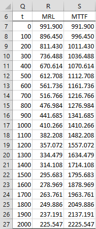
Figure 3 – Mean Residual Life

We see that as t gets larger, MLE(t) gets smaller but MTTF(t) gets larger, as you would expect.

Examples Workbook

Click here to download the Excel workbook with the examples described on this webpage.

References

Wikipedia (2012) Weibull distribution
https://en.wikipedia.org/wiki/Weibull_distribution

McCool, J. I. (2012) Using the Weibull distribution: reliability, modeling and inference. Wiley
https://fac.ksu.edu.sa/sites/default/files/john_i._mccoolauth._using_the_weibull_distribub-ok.xyz_.pdf

Morris, S. (2023) Conditional Weibull distribution
https://reliabilityanalyticstoolkit.appspot.com/conditional_weibull_distribution