Basic Concepts
The pdf of the Pareto (type I) distribution with scale parameter m > 0 and scale parameter α > 0 is
![]()
for x ≥ m and f(x) = 0 otherwise. The corresponding cumulative distribution is
![]()
for x ≥ m and F(x) = 0 otherwise.
From the formula for the cdf, it is easy to see that the inverse function is
![]()
Properties
Key statistical properties of the Pareto distribution are shown in Figure 1.

Figure 1 – Statistical properties of the Pareto distribution
For a graph of the Pareto distribution at m = 1 and α = 1, 2, 3, see Figure 2.
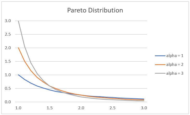
Figure 2 – Pareto distribution
Worksheet Functions
Real Statistics Functions: The Real Statistics Resource Pack provides the following functions for the Pareto distribution.
PARETO_DIST(x, α, m, cum) = pdf of the Pareto distribution f(x) when cum = FALSE and the corresponding cumulative distribution function F(x) when cum = TRUE.
PARETO_INV(p, α, m) = inverse of the Pareto distribution at p.
Distribution Fitting
Given a collection of data that may fit the Pareto distribution, we explore two ways to estimate the parameters that best fit the data. See the following for details: Method of Moments and MLE Fitting.
Pareto Principle
In the case where the shape parameter is α = log45 = 1.160964, we get the famous Pareto principle, aka the 80-20 rule, which states that 80% of the outcomes are due to 20% of the causes. E.g. 20% of the workers do 80% of the work. 80% of the wealth is owned by 20% of the people.
Generalized Pareto Distribution
Click here for information about a generalization of the Pareto distribution.
Examples Workbook
Click here to download the Excel workbook with the examples described on this webpage.
References
Wikipedia (2021) Pareto distribution
https://en.wikipedia.org/wiki/Pareto_distribution
Wikipedia (2021) Pareto principle
https://en.wikipedia.org/wiki/Pareto_principle