When data is missing in a time series, we can use some form of imputation or interpolation to impute a missing value. In particular, we consider the approaches described in Figure 1.
| Numeric label | Text label | Imputation type |
| 0 | linear | linear interpolation |
| 1 | spline | spline interpolation |
| 2 | prior | use prior value |
| 3 | next | use next value |
| -1 | sma | simple moving average |
| -2 | wma | weighted moving average |
| -3 | ema | exponential moving average |
Figure 1 – Imputation Approaches
Example
Example 1: Apply each of these approaches for the time series with missing entries in column E of Figure 2. The full time series is shown in column B.
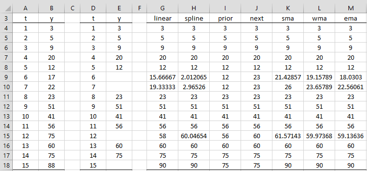
Figure 2 – Imputation Examples
Linear interpolation
The missing value in cell E15 is imputed as follows as shown in cell G15.
![]()
The missing value in cell E10 is imputed as follows as shown in cell G10.
![]()
Finally, the missing value in cell E18 is imputed as follows as shown in cell G18.
![]()
Spline interpolation
To create the spline interpolation for the four missing values, first, create the table in range O3:P14 by removing all the missing values. This can be done by placing the array formula =DELROWBLANK(D3:E18,TRUE) in range O3:P14, as shown in Figure 3. Next place the array formula =SPLINE(R4:R18,O4:O14,P4:P14) in range S4:S18 (or in range H4:H18 of Figure 2).
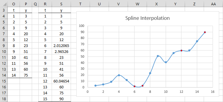
Figure 3 – Spline interpolation
The chart of the spline curve is shown on the right side of Figure 3. The imputed values are shown in red on the chart.
See Spline Fitting and Interpolation for additional information.
Prior/Next
For Next the next non-missing value is imputed (or the last non-missing value if there is no next non-missing value), while for Prior the previous non-missing value is imputed (or the first non-missing value if there is no previous non-missing value).
The missing value in cell E9 is imputed as 23 (cell J9) when using Next and 12 (cell I9) when using Prior. The missing value in cell E18 is imputed as 75 (cell I18 or J18) when using Prior or Next.
Simple Moving Average
The imputed value depends on the span value k which is a positive integer. To impute the missing values, we first use linear interpolation, as shown in column AE of Figure 4. For any missing values in the first or last k elements in the time series, we simply use the linear interpolation value. For the others, we use the mean of the 2k+1 linear interpolated values on either side of the missing value.
In Figure 2 we use a span value of k = 3. To show how the values in column K of Figure 2 are calculated, we calculate the linear interpolated values as shown in column AE of Figure 4. Next, we place the formula =IF(AD4=””,AE4,AD4) in cell AF4, highlight range AF4:AF6 (i.e. a column range with k = 3 elements) and press Ctrl-D. Similarly, we copy the formula in cell AF4 into the last 3 cells in column F.
Next, we place the formula =IF(AD7=””,AVERAGE(AE4:AE10),AD7) in cell AF7, highlight the range AF7:AF15 (i.e. all the cells in column AF that haven’t yet been filled in), and press Ctrl-D. The imputation should in column K is identical to that shown in column AF.
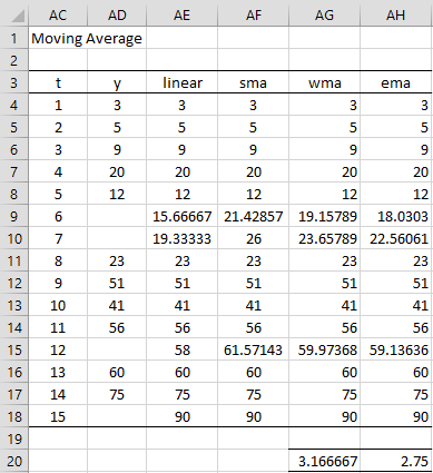
Figure 4 – Moving Average Imputations
Weighted Moving Average
The approach is similar to the simple moving average approach, except that now weights are used. For example, the first missing time series element occurs at time t = 6. Thus, we weight the linear imputed values in column AE of Figure 4 by 1 for t = 6, by 1/2 for t = 5 or 7, by 1/3 for t = 4 or 8, and by 1/4 for t = 3 or 9. The calculation of the imputed value at t = 6 is shown in Figure 5.
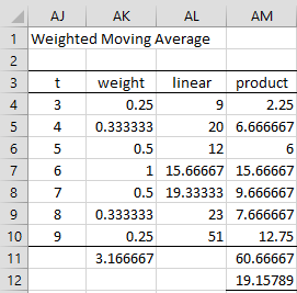
Figure 5 – WMA for t = 6
Here, cell AK4 contains the formula =1/(ABS(AJ$7-AJ4)+1), cell AL4 contains =AE6 and cell AM4 contains =AK4*AL5. We can now highlight the range AK:AM10 and press Ctrl-D to fill in the other values. Then we sum the weights to obtain the value 3.16667 as shown in cell AK11 and sum the products to obtain the value 60.66667 as shown in cell AM11. The imputed value is thus 60.66667 divided by 3.166667, i.e. 19.15789 as shown in cell AM12.
This is the value shown in cell AG9 of Figure 4. In fact, we can fill in column AG of Figure 4 as follows. First, insert the worksheet formula =1+2*SUMPRODUCT(1/AC5:AC7) in cell AG20. Next, fill in the first 3 and last 3 values in column AG by using the values in column AE. Finally, insert the following formula in cell AG7, highlight range AG7:AG15, and press Ctrl-D.
=IF(AD7=””,SUMPRODUCT(AE4:AE10,1/(ABS(AC4:AC10-AC7)+1))/AG$20,AD7)
Exponential (Weighted) Moving Average
The approach is identical to that of the weighted moving average except that we use weights that are a power of 2. Now, we weight the linear imputed values in column AE of Figure 4 by 1 for t = 6, by 1/2 for t = 5 or 7, by 1/4 for t = 4 or 8, and by 1/8 for t = 3 or 9.
The calculation of the imputed value at t = 6 is as shown in Figure 5, except that the formula used for cell AK4 is now =1/2^ABS(AJ$7-AJ4) (and similarly for the other cells in column AK). The result is as shown in column AH of Figure 4. This time, cell AH7 contains the formula
=IF(AD7=””,SUMPRODUCT(AE4:AE10,1/2^ABS(AC4:AC10-AC7))/AH$20,AD7)
and cell AH20 contains the formula =1+2*SUMPRODUCT(1/2^AC4:AC6).
Worksheet Function
Real Statistics Function: For a time series represented as a column array where any non-numeric values are treated as missing, the Real Statistics Resource Pack supplies the following array function:
TSImputed(R1, itype, k): returns a column array of the same size as R1 where each missing element in R1 is imputed based on the imputation type itype which is either a number or text string as shown in Figure 2 (default 0 or “linear”) and k = the span (default 2), which is only used with the three moving average imputation types.
For example, =TSImputed(E4:E18,”ema”,3) returns the time series shown in range M4:M18 of Figure 2.
Seasonality
If the time series has a seasonal component, then we can combine one of the imputation approaches described in Figure 1 with a seasonality imputation approach as described in Handling Missing Seasonal Time Series Data.
Examples Workbook
Click here to download the Excel workbook with the examples described on this webpage.
References
Geeks for Geeks (2023) How to deal with missing values in a timeseries in Python?
https://www.geeksforgeeks.org/how-to-deal-with-missing-values-in-a-timeseries-in-python/
Kusawa, S. (2023) Handle missing values in time series datasets: 10 best techniques
https://datamagiclab.com/handle-missing-values-in-time-series-datasets/