Definitions
Definition 1: The autocorrelation function (ACF) at lag k, denoted ρk, of a stationary stochastic process, is defined as ρk = γk/γ0 where γk = cov(yi, yi+k) for any i.
Note that γ0 is the variance of the stochastic process.
Definition 2: The mean of a time series y1, …, yn is

The autocovariance function at lag k, for k ≥ 0, of the time series is defined by
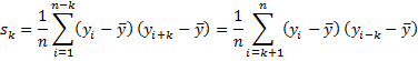
The autocorrelation function (ACF) at lag k, for k ≥ 0, of the time series is defined by
![]()
The variance of the time series is s0. A plot of rk against k is known as a correlogram. See Correlogram for information about the standard error and confidence intervals of the rk, as well as how to create a correlogram including the confidence intervals.
Observation: The definition of autocovariance given above is a little different from the usual definition of covariance between {y1, …, yn-k} and {yk+1, …, yn} in two respects: (1) we divide by n instead of n–k and we subtract the overall mean instead of the means of {y1, …, yn-k} and {yk+1, …, yn} respectively. For values of n which are large with respect to k, the difference will be small.
Example
Example 1: Calculate s2 and r2 for the data in range B4:B19 of Figure 1.

Figure 1 – ACF at lag 2
The formulas for calculating s2 and r2 using the usual COVARIANCE.S and CORREL functions are shown in cells G4 and G5.
The formulas for s0, s2, and r2 from Definition 2 are shown in cells G8, G11, and G12 (along with an alternative formula in G13). Note that the values for s2 in cells E4 and E11 are not too different, as are the values for r2 shown in cells E5 and E12; the larger the sample the more likely these values will be similar.
Worksheet Functions
Real Statistics Functions: The Real Statistics Resource Pack supplies the following functions for column array or range R1:
ACF(R1, k) = the ACF value at lag k for the time series in R1
ACVF(R1, k) = the autcovariance at lag k for the time series in R1
Note that ACF(R1, k) is equivalent to
=SUMPRODUCT(OFFSET(R1,0,0,COUNT(R1)-k)-AVERAGE(R1),OFFSET(R1,k,0,COUNT(R1)-k)-AVERAGE(R1))/DEVSQ(R1)
Observations
There are theoretical advantages to using division by n instead of n–k in the definition of sk, namely that the covariance and correlation matrices will always be definite non-negative (see Positive Definite Matrices).
Even though the definition of autocorrelation is slightly different from that of correlation, ρk (or rk) still takes a value between -1 and 1, as we see in Property 2.
Properties
Property 1: For any stationary process, γ0 ≥ |γi| for any i
Proof: Click here
Property 2: For any stationary process, |ρi| ≤ 1 (i.e. -1 ≤ ρi ≤ 1) for any i > 0
Proof: By Property 1, γ0 ≥ |γi| for any i. Since ρi = γi /γ0 and γ0 ≥ 0 (actually γ0 > 0 since we are assuming that ρi is well-defined), it follows that
![]()
Example with Correlogram
Example 2: Determine the ACF for lag = 1 to 10 for the Dow Jones closing averages for the month of October 2015, as shown in columns A and B of Figure 2, and construct the corresponding correlogram.
The results are shown in Figure 2. The values in column E are computed by placing the formula =ACF(B$4:B$25, D5) in cell E5, highlighting range E5:E14 and pressing Ctrl-D.

Figure 2 – ACF and Correlogram
As can be seen from the values in column E or the chart, the ACF values descend slowly towards zero. This is typical of an autoregressive process.
Observation: A rule of thumb is to carry out the above process for lag = 1 to n/3 or n/4, which for the above data is 22/4 ≈ 6 or 22/3 ≈ 7. Our goal is to see whether by this time the ACF is significant (i.e. statistically different from zero). We can do this by using the following property.
Tests
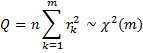
Property 3 (Bartlett): In large samples, if a time series of size n is purely random then for all k
![]()
Example 3: Determine whether the ACF at lag 7 is significant for the data from Example 2.
As we can see from Figure 3, the critical value for the test in Property 3 is .417866. Since r7 = .031258 < .417866, we conclude that ρ7 is not significantly different from zero.

Figure 3 – Bartlett’s Test
Note that using this test, values of k up to 3 are significant and those higher than 3 are not significant (although here we haven’t taken experiment-wise error into account).
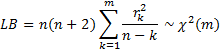
Property 4 (Box-Pierce): In large samples, if ρk = 0 for all k ≤ m, then
A more statistically powerful version of Property 4, especially for smaller samples, is given by the next property.
Property 5 (Ljung-Box): If ρk = 0 for all k ≤ m, then
Example 4: Use the Box-Pierce and Ljung-Box statistics to determine whether the ACF values in Example 2 are statistically equal to zero for all lags less than or equal to 5 (the null hypothesis).
The results are shown in Figure 4.

Figure 4 – Box-Pierce and Ljung-Box Tests
We see from these tests that ACF(k) is significantly different from zero for at least one k ≤ 5, which is consistent with the correlogram in Figure 2.
Test worksheet functions
Real Statistics Functions: The Real Statistics Resource Pack provides the following functions to perform the tests described by the above properties.
BARTEST(r, n, lag) = p-value of Bartlett’s test for correlation coefficient r based on a time series of size n for the specified lag.
BARTEST(R1,, lag) = BARTEST(r, n, lag) where n = the number of elements in range R1 and r = ACF(R1,lag)
PIERCE(R1,,lag) = Box-Pierce statistic Q for R1 and the specified lag
BPTEST(R1,,lag) = p-value for the Box-Pierce test for R1 and the specified lag
LJUNG(R1,,lag) = Ljung-Box statistic Q for R1 and the specified lag
LBTEST(R1,,lag) = p-value for the Ljung-Box test for R1 and the specified lag
In the above functions, R1 is a column array or range.
Where the second argument is missing, the test is performed using the autocorrelation coefficient (ACF). If the value assigned instead is 1 or “pacf” then the test is performed using the partial autocorrelation coefficient (PACF) as described in the next section. Actually, if the second argument takes any value except 1 or “pacf”, then the ACF value is used.
For example, BARTEST(B4:B25,,7) = BARTEST(.031258,22,7) = .441718 for Example 3 and LBTEST(B4:B25,”acf”,5) = 1.81E-06 for Example 4.
Examples Workbook
Click here to download the Excel workbook with the examples described on this webpage.
References
Greene, W. H. (2002) Econometric analysis. 5th Ed. Prentice-Hall
https://www.ctanujit.org/uploads/2/5/3/9/25393293/_econometric_analysis_by_greence.pdf
Gujarati, D. & Porter, D. (2009) Basic econometrics. 5th Ed. McGraw Hill
http://www.uop.edu.pk/ocontents/gujarati_book.pdf
Hamilton, J. D. (1994) Time series analysis. Princeton University Press
https://press.princeton.edu/books/hardcover/9780691042893/time-series-analysis
Wooldridge, J. M. (2009) Introductory econometrics, a modern approach. 5th Ed. South-Western, Cegage Learning
https://cbpbu.ac.in/userfiles/file/2020/STUDY_MAT/ECO/2.pdf
Dr Zaionit good evening, Dr. there is an error in the example:
BARTEST(.303809,22,7) = .07708
Is not correct 0.30…, the correct is B4:B25
Etc.
Thanks
Hello Gerardo,
Good to see a comment from you and thank you very much for catching this error.
I believe that I have corrected the error. Please let me know if this is not correct or you find another error.
Charles
Série AG h aux1 aux2 FAC Plug-in ==>IC [-0,207; 0,2066]
0,80 -0,360028732 0 91 2 1 Values >0,207 and
0,81 -0,347528732 1 90 3 0,48 (0,23 ) < -0,207 are the
0,81 -0,347528732 2 89 4 0,43 (0,18) significant lags.
1,11 -0,048917621 3 88 5 0,25 (0,06) In this exempla
0,53 -0,632250954 4 87 6 0,11 k=1 explain 23%
0,81 -0,347528732 5 86 7 0,06 of results and
1,42 0,261023899 6 85 8 -0,09 k=2 explain 18%
1,33 0,173304601 7 84 9 -0,20
1,73 0,567243995 8 83 10 -0,20
0,81 -0,347528732 9 82 11 -0,21
1,20 0,039971268 10 81 12 -0,14
1,33 0,173304601 11 80 13 -0,29 0,08
1,22 0,06219349 12 79 14 -0,15
1,22 0,06219349 13 78 15 -0,14
1,20 0,039971268 14 77 16 -0,07
1,67 0,506637934 15 76 17 -0,04
1,60 0,439971268 16 75 18 -0,06
1,36 0,197114125 17 74 19 -0,14
2,15 0,993817422 18 73 20 -0,07
1,08 -0,083105655 19 72 21 -0,04
2,09 0,930880359 20 71 22 -0,08
1,81 0,652471268
1,92 0,763048191
0,90 -0,260028732
0,81
Nice and it is helpful information to understand the concept of Auto-correlation and calculation
Hi Charles,
Great website. So much truly useful information.
I am wondering if you can please point me in the right direction.
I am trying to understand how to properly quantify autocorrelation for serial data with missing data points. I have conducted an experiment where I created a sequence of random numbers (310 in total) and then created a set with some data randomly removed (data set 1: 119 removed). When I look at your ACF and Pearson/Correl values from Excel I get very similar numbers. I understand the population/sample size isn’t quite the same so there is a small difference between them Check. Now, when I apply the same procedure to the array of data with missing entries your ACF and the Pearson/Correl are quite different in appearance and scale? What is the correct way to calculate the ACF for serial data missing data points?
Thanks,
David
David,
If you are using random numbers to create a set X with 310 elements, then I would expect little autocorrelation. If you remove 119 data elements randomly to create set Y, then the data should still be randomly distributed and once again the autocorrelation should be close to zero.
The value of Pearson/Correl depends on which two sets you are using. If you are using X and Y, you can’t calculate the correlation since they don’t have the same number of elements. If instead, you remove any element from X that was missing in Y, then of course the two sets will be identical and the correlation will be 1. Different arrangements will yield different correlations.
Charles
Hi Charles,
I am a little bit confused when you said that: “you can’t calculate the correlation since they (a full set of X and a shorten set of Y) don’t have the same number of elements.”. There are an analytical method known as Convolution Function and this Convolution Function can be computed for any 2 sets of data with or without having the same number of elements with a number of lags you want to define. Once this Convolution Function is obtained, you can easily calculate the Auto-Correlation Function for 2 sets of data.
Hi Nikolai,
I am a little confused as to what you are looking for. If you have two sets X and Y, then you can discuss the correlation between these sets. When you have one set X (or Y) then you can speak about autocorrelation. With two sets X and Y, you can speak about autocorrelation if you can combine the two sets in some reasonable way, e.g. when both refer to time and so you can order the combined set into one time series. In this case, it doesn’t matter whether X and Y have the same number of elements.
Charles
Hi Charles,
All I am trying to say is that, if you have 2 sets of data with unequal data of points, you can find the correlation between 2 sets of data using the method known as Convolution. The bottom line is, the correlation of 2 sets of data can be computed and it does not require the 2 sets must have the same number of data points. If somehow my previous message confused you, accept my apology because I may explain my point not clear enough :-).
Nikolai,
As explained in my last comment, this is true for autocorrelation. I don’t believe that this is true for Pearson’s correlation.
Charles
Can someone explain why I get different results when I use CORREL and sum product methods to find auto-correlation of a data set and which one is right?
Dasun,
The formulas are slightly different. If you use the formula for ACF, the denominator is s_0, which is based on the whole sample. If you use CORREL the denominator will be slightly different since it is based on a smaller sample. Technically, I would say that the version based on CORREL is right, but the ACF formula is the one that is commonly used and probably makes the mathematics come out better.
Charles
Dear Charles
I tried to use your Correlogram data analysis tool but I was not able to undertsand why you chose to fix at 60 the maximum number of lags.
Could you give me some explanations?
All the best.
Lorenzo Cioni
Lorenzo,
It was a relatively arbitrary limit. What maximum value is best for you?
Charles
Charles
I don’t think of a best value but rather of a value linked in some way with the available amount of data so that if I have an array of N values the maximum lag could be a value lower than N but such that the calculations are meaningful. This fact is linked to what I asked you in my previous message, the one of April 27, 2020 at 10:20 am.
Lorenzo
Thanks for the suggestion, Lorenzo. I will look into this.
Charles
Dear Charles
in the Observation you write “For values of n which are large with respect to k, the difference will be small.” What if k is almost equal to n? There is any limit of the value of k with regad to the value of n? or to be more clear there is a relation between the value of n and the upper value of k?
Thank you in advance.
All the best.
Lorenzo
The lagged correlation and the lagged autocorrrelation have the same symbol “r2” and similarly for the variance. As a beginner, this created some confusion. But, overall, thanks for putting this up.
Hi, how did you calculate autocorrelation for each lag?
Hello Rami,
This is described on this webpage. Do you have a specific question about how the calculation was made?
Charles
Hi, in determining the ACF for lag = 1 to 10, where did you find the formula =ACF(B$4:B$25,D5) in Excel? Can’t find it in excel formulas. (Excel 2013).
I think you are confused when you tried to read and follow instructions from Charles’s webpage. If you want to use the built-in ACF function in Excel and you can just enter the formula = ACF(B$4:B$25,D5) to call out the ACF function as Charles said, you need to install the analysis tool package known as NumXL. However, this analysis tool package is not for free to download and install in your Excel. If you don’t have this NumXL installed, this function ACF is not available in your Excel worksheet to call it out. So having said all that, without having NumXL, in your Excel worksheet, if you want to calculate the ACF, you need to enter the entire formula =SUMPRODUCT(OFFSET(R1,0,0,COUNT(R1)-k)-AVERAGE(R1),OFFSET(R1,k,0,COUNT(R1)-k)-AVERAGE(R1))/DEVSQ(R1)
where R1 is representing the entire range of your data set and k is the lag number.
Hi Charles and Nikolai,
Thank you a lot for this convenient replacement! But unfortunately I can’t get the same values for ACF as shown in the example provided here – Correlogram, Figure 1, https://real-statistics.com/time-series-analysis/stochastic-processes/correlogram/. Sure, I use exactly the same raw data as shown there.
To replace ACF by the equivalent, I write the following formula to D7 cell (similar to that Figure), where R1 = A$4:A$59 (entire range of data):
=SUMPRODUCT(OFFSET(A$4:A$59;0;0;COUNT(A$4:A$59)-C7)-AVERAGE(A$4:A$59);OFFSET(A$4:A$59;C7;0;COUNT(A$4:A$59)-C7)-AVERAGE(A$4:A$59))/DEVSQ(A$4:A$59))
And the D8 is (I just replace C7 reference to C8 here):
=SUMPRODUCT(OFFSET(A$4:A$59;0;0;COUNT(A$4:A$59)-C8)-AVERAGE(A$4:A$59);OFFSET(A$4:A$59;C8;0;COUNT(A$4:A$59)-C8)-AVERAGE(A$4:A$59))/DEVSQ(A$4:A$59))
And so on for D9, D10, etc.
However, the value of D7 is 0.7182, not 0.8742. Definitely, I made an error but I can’t get the idea where I did it. I would appreciate so much your help!
My apologizes, I solved the issue! It was my mistake with correct filling of the raw data range. Please don’t respond to the previous question. Thanks a lot!
Hi I got it now,, reply not needed.
But in the covariance formula in excel divide by n–k(18-1=17 in this case) subtract individual means of {y1, …, yn-k} and {yk+1, …, yn} respectively instead of the total mean.
I see this contradicts with what you have mentioned under observation.
Hello Ranfer,
Yes, this will be different from the COVARIANCE.S, COVARIANCE.P and CORREL formulas in Excel.
Charles
Understood, btw Sir, Do you plan to include an explanation over ARCh & GARCH models as well any time soon ?
Hello Ranil,
Yes. This capability won’t be in the next release, but I expect to add it in one of the following releases.
Charles
Hi,
To calculate the critical Value for the Ljung-Box test, I do not understand why you divide alpha (5%) by two (Z5/2) ; (=CHISQ.INV.RT(Z5/2,Z4)).
Thank you.
Hi Raji,
I don’t understand either. I have corrected this error. Thanks for identifying this mistake.
Charles
Hi,
The results i got have acf, t-stat and p value…could u please help with the interpretation of the same.
Thanks
Neha
Dr Neha,
Which test are you referring to? I don’t believe that any of the tests on this webpage use the t stat
Charles
In “Figure 4 – Box-Pierce and Ljung-Box Tests” in cell AB7 it should be
SUMPRODUCT((E5:E9)^2/(Z3-D5:D9)) if it references to “Figure 2 – ACF and Correlogram”
So instead of D and C it is E and D.
Dirk,
Thanks for identifying this error. I have now corrected the figure on the webpage.
I really appreciate your help in improving the accuracy and quality of the website.
Charles
“Equations of the form p(k)~Ak^(-\alpha) should be shown”. Is this related to ACF ? How
Sorry, but I don’t understand your comment. What is A? What is the equation?
Charles
Hi
in the link bellow i put the true test of ACP and PACF to identify ARMA and SARMA orders. This is what we expect the Real statistics show us when we testing a time series.
in this workbook i provided the bounds of ACF and PACF significance just like Shazam, EViews and Stata.
Sohrab,
Thanks for sending this to me. I will investigate your suggestions.
Charles
I have investigated this matter further and will include the Correlogram in the next release of the Real Statistics software. This should be available in a couple of days. Thanks again for your suggestion.
Charles
Hi,
In your note
“Note that values of k up to 5 are significant and those higher than 5 are not significant.”
I don’t understand why is it up to 5. According to the text:
If ACF k is not significant
Under this rule I see that just values of k until 3 are significant.
Did I missunderstand something?
Don’t know why but the symbols don’t appear in my comment but I said that according to the text:
If the ACF is lower than the critic value for any lag k, then it is not significant.
This would imply that just lag 1 to 3 are significant.
Is this correct?
Using for definition lags values for analysis:
k =10*LOG10(n)
For exemplo: n = 90 , so k= 19,54 ~20
Jairo,
Yes, you are correct. The webpage should say 3 instead 5. Thanks for catching this error. I have now corrected this. I think that 5 referred to a previous version of the example. Thanks for improving the accuracy of the website.
Charles
Hi,
I do not understand in Figure 3 the Content of cell P8 (0.303809) which Comes from cell D11 respectively I cannot trace it back to the examples further above.
your help is much appreciated.
Dan,
The problem is that I changed some values, but did not update the figure. I have now corrected the error and so you should be able to figure out how to trace each cell.
Thanks for discovering this error. I appreciate your help in improving the website and sorry for the inconvenience.
Charles
Dear Charles,
How do we say ACF values are significant by PIERCE(R1,,lag) and LJUNG(R1,,lag)? Can you please explain with the example2 ACF values?
I got it and I understand. Reply not needed
Thank you
Sreepada