Positive and null recurrence
Suppose i is a recurrent state (see Connectivity). i is positive recurrent if ni < ∞ and null recurrent if ni = ∞ (see Hitting Probabilities for the definition of ni).
Property 1: In a recurrent class, all states are positive recurrent or all states are null recurrent.
Proof: The proof is similar to that of Property 4 of Connectivity.
Property 2: In a finite closed class, all states are positive recurrent.
Proof: The proof is similar to that of Property 7 of Connectivity.
Based on these properties and related properties in Connectivity, we observe that
- Non-closed classes are transient
- Closed classes in finite Markov chains are positive recurrent
- Closed classes in infinite Markov chains can be transient, null recurrent or positive recurrent.
As we observe in Connectivity, for a one-dimensional random walk with p ≠ .5, all states are transient. When p = .5 all states are recurrent, but as we observe in Random Walks, n0 = ∞, and so all states are null recurrent.
Existence/uniqueness of a stationary distribution
Property 3: For an irreducible Markov chain
- If the chain is positive recurrent, then a unique stationary distribution π exists where πi = 1/ni, where ni is the expected time to return to state i.
- If the chain is null recurrent or transient, then no stationary distribution exists
Note that even if the Markov chain is not irreducible, Property 3 applies to any communications class that is positive recurrent (and so is closed). The unique stationary distribution applies only to that class.
By Property 7 of Connectivity, a finite, irreducible Markov chain is always positive recurrent, and so Property 3 holds.
Stationary distribution example
Example 1: Find the stationary distribution for the transition matrix in range B2:D4 of Figure 1.
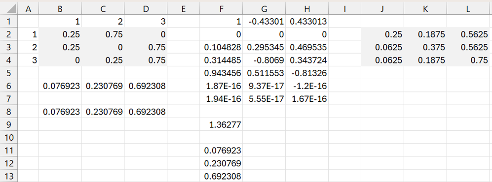
Figure 1 – Stationary distribution
First note that the formula =MPOWER(B2:D4,2) yields the matrix in range J2:L4. Since all the elements in this matrix are positive, per Property 4 of Markov Chain Distributions, there is a unique stationary distribution. This distribution is displayed in range B6:D6, using the approach described in Markov Chain Distributions. We see that the formula =MMULT(B6:D6,B2:D4) yields the results shown in range B8:D8, namely (1/13, 3/13, 9/13),
We note that 1 ↔ 2 ↔ 3, and so the chain is irreducible. Since the Markov chain is finite and there is one communications class, by Property 7 of Connectivity, it is recurrent, and so ti = 1 for i = 1, 2, 3.
We can calculate n11, n22, and n33, as described in Hitting Probabilities.
Calculating n11
k31 = 1 + .25 k21 + .75 k31
.25 k31 = 1 + .25 k21
k31 = 4 + k21
k21 = 1 + .25 k11 + .75 k31 = 1 + .25(0)+ .75(4+k21)
.25 k21 = 1 + 3
k21 = 4(4) = 16
n11 = 1 + .25 k11 + .75 k21 = 1 + .25(0)+ .75(16) = 13
The calculation for n22 is as follows
Under construction
Thus, per Property 3, the chain is positive recurrent.
References
Aldridge, M. (2021) Recurrence and transience. Introduction to Markov Processes
https://mpaldridge.github.io/math2750/S09-recurrence-transience.html
Norris, J. (2004) Discrete-time Markov chains. Cambridge University Press
https://www.statslab.cam.ac.uk/~jrn10//Markov/