Panel Data over Two Time Periods

Data formats

We now consider the case where we have data for the same units in two time periods. We have a few choices for how to represent the data. Suppose that we are interested in how the crime rate (cases per 100,000 people) is affected by the unemployment rate (0-100%) and possibly also population size (in thousands of inhabitants). In particular, we are interested in how this relationship changes from 1992 to 1998. We use the data for 8 different cities as shown in Figure 1.

Balanced Panel

Since for each unit, we have data for both time periods, we have a balanced panel. The data is sorted first by unit (city) and then by time period (year). Data in this format is easiest to process and so we will assume that the panel data that we analyze will be in this format. In fact, if we know that there are two time periods and that we have balanced data, often it will be sufficient for our purposes to omit columns A and B and use columns C, D, and E only.

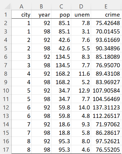
Figure 1 – Panel data

Note that if the data is not in the order displayed in Figure 1, they can be sorted to obtain this format.

Regression models

Using the type of data shown in Figure 1, we want to determine how the crime rate is affected by unemployment and possibly population size. In particular, we want to see how this relationship changes from 1992 to 1998. We can use the regression model

Here, crime_it, unem_it and e_it take both a cross-sectional subscript i, representing a city, and a time subscript t, representing 1992 or 1998. pop_i only takes a cross-sectional subscript since the population data in column C is based on census data and so doesn’t change from 1992 to 1998. The fact that this data is time-invariant will turn out to be relevant in how we analyze the panel data.

Actually, the crime rate is potentially influenced by many factors that are not included in this model. In particular, these may include a time-constant factor such as the city’s location. It may also include demographic factors (mean age, racial profile, etc.) that are assumed not to change over time.

We can add these factors to the model to reduce the size of the error component e_it. It may indeed be necessary to add such factors so that the model is not under-specified, especially when this results in a violation of the regression assumptions (e.g. to avoid e_it being correlated with one or more of the independent variables).

Using an unobserved effect

Instead of adding such factors, we will add an unobserved (time-invariant) effect u_i, resulting in the model

Since we have no data for u_i, how can we estimate the values of the regression coefficients? One approach is to include u_i in the error term to obtain a composite error term v_it = u_i + e_it and use OLS regression. In fact, we will adopt this approach subsequently when considering the random-effects model (REM).

Often, however, this approach is not appropriate since if u_i is correlated with one or more of the independent variables (unem_it in our example), then v_it will also be correlated with unem_it, which violates an OLS regression assumption. In this case, we need to use a regression model that is valid even when the unobserved variable is correlated with one or more of the independent variables (by differencing or demeaning).

Examples Workbook

Click here to download the Excel workbook with the examples described on this webpage.

References

Gujarati, D. & Porter, D. (2009) Basic econometrics. 5th Ed. McGraw Hill
http://www.uop.edu.pk/ocontents/gujarati_book.pdf

Hill, R. C., Griffiths, W. E., Lim, G. C. (2018) The principles of econometrics. 5^th edition. Wiley.