Basic Concepts
We now demonstrate a third approach to creating a fixed-effects model for panel data. It turns out that this approach, called the Least-squares Dummy Variable (LSDV), is equivalent to the demeaning approach. This approach has the advantage that it is intuitively clearer and doesn’t require any adjustments to the standard errors. It has the disadvantage, however, of requiring the addition of new dummy variables, one for each unit, which, especially when the number of units is large, makes the model a bit unwieldy.
Example
Example 1: Repeat Example 1 of Differencing for Panel Data using the LSDV approach.
This model is created by adding dummy variables for the units. You have two choices: (1) add one dummy variable for each unit but omit the intercept, or (2) add one variable for all but one variable and include an intercept. Choosing approach (1), we obtain the model shown in Figure 1.
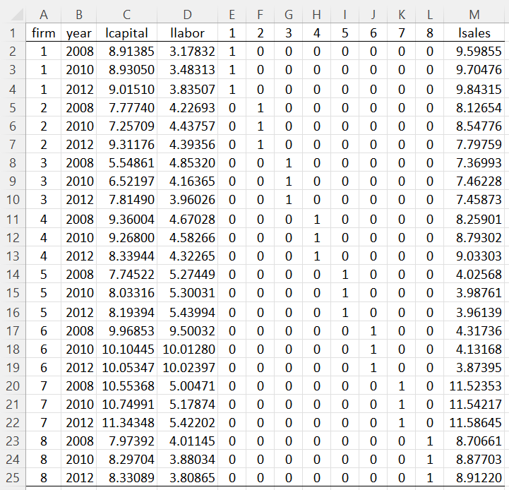
Figure 1 – Dummy Variable Model
Here, we insert the formula =IF($A2=E$1,1,0) in cell E2, highlight the range E2:L25, and press Ctrl-R and Ctrl-D. We then perform OLS regression to obtain the output shown in Figure 2.
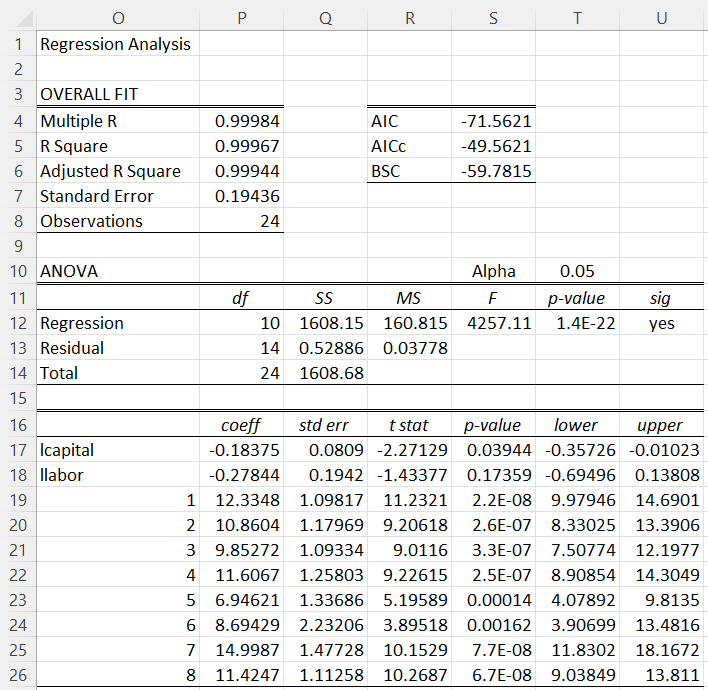
Figure 2 – LSDV regression
We see that the results for lcapital and llabor in Figure 2 are the same as those in Figure 3 of Demeaning for Panel Data.
Worksheet Function
Real Statistics Function: The Real Statistics Resource Pack provides the following worksheet function where R1 contains balanced panel data sorted first by unit and then by time period with the data for the dependent variable in the last column, as in columns C, D, and E of Figure 1 of Demeaning for Panel Data (equivalent to columns C, D, and M of Figure 1).
PANEL_DVM(R1, periods, head, ttype): returns an array with the unit means for the data in R1 based on periods number of time periods
If head = TRUE (default FALSE) then it is assumed that the panel data contains column headings and that these will be used to create column headings for the output.
When ttype = 0 (default), then one dummy variable is added for each unit. If ttype = 1 then one dummy variable is added for each unit, omitting the first unit (the baseline). If ttype = -1 then one dummy variable is added for each unit, omitting the last unit (the baseline).
Thus, we obtain the data in Figure 1 by using the formula =PANEL_DVM(C1:E25,3,TRUE) where C1:E25 refers to the data in Figure 1 of Demeaning for Panel Data.
Differences between Units
To determine whether there are differences between the different firms, we need to test the null-hypothesis
H0: d1 = d2 = ⋅⋅⋅ = d8.
As usual, using the formula =Rsquare_Test(C2:L25,C2:D25,M2:M25,TRUE), whose output is shown in Figure 3, we see there are significant differences between the firms.
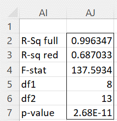
Figure 3 – R-square Test
Examples Workbook
Click here to download the Excel workbook with the examples described on this webpage.
Links
References
Gujarati, D. & Porter, D. (2009) Basic econometrics. 5th Ed. McGraw Hill
http://www.uop.edu.pk/ocontents/gujarati_book.pdf
Hill, R. C., Griffiths, W. E., Lim, G. C. (2018) The principles of econometrics. 5th edition. Wiley.
I am applying difference-in-difference regression for panel data using Excel and your examples as a template since my data was too complex to code for in R even with R experts. Thanks so much for these tutorials!
Hello Jacob,
Glad I could help.
Charles
Hi Charles,
That is very helpful thank you.
I’ve been grappling with the matter of adding country and time dummy variables to a time series model of my own, since I’ve seen it being stated as useful and/or necessary to “absorb” country and time variations. [One such paper is: Market forces and workers’ power resources: A sociological account of real wage growth in advanced capitalism – see the regression results table on page 111.]
I’ve found, however that when I add country and time dummy variables on top of the existing variables, that variance inflation goes through the roof. This is the case for OLS – I’ve not attempted it yet with FE but I will shortly. Thus far however, either I’m not doing it correctly, or the model is not amenable to dummy variables. Do you have any experience of this, that the addition of country and time dummy variables produces untenable variance inflation (VIF>10)?
Then, where the LSDV model on this page clearly includes dummy variables, I wonder whether this would satisfy the expectation for inclusion of country dummy variables? Then all that is needed is for time dummy variables to be added.
Thank you,
Gareth
Hi Gareth,
You can certainly add dummy variables, but you also need to make sure the regression assumptions are met. Also adding dummy variables uses up degrees of freedome.
Charles
Hello Charles,
Regarding the function PANEL_DVM.
If ttype is either 1 or -1, how does that affect the output and how are the coefficients interpreted?
Thank you
Gareth
Hello Gareth,
If ttype = 1 then there are 7 dummy variables 2, 3, 4, 5, 6, 7, 8 (1 is the reference variable). If ttype = -1 then the 7 dummy variables are 1, 2, 3, 4, 5, 6, 7 (8 is the reference variable). In either of these cases regression with intercept is used. The intercept coefficient is equal to the reference coeffcient in the model where ttype = 0. If you add the intercept coeffcient in the ttype = -1 case to each of the other dummy coefficients you get the dummy coefficients from the ttype = 0 model. If you subtract the intercept coeffcient in the ttype = 1 case from each of the other dummy coefficients you get the dummy coefficients from the ttype = 0 model.
I have also updated this webpage to include the spreadsheet with the worksheet displayed on the webpage (the ttype = 0 case). I have also added two additional worksheets with the ttype = 1 and -1 cases.
Charles