Differencing Models over Two Time Periods

Basic Concepts

One approach to dealing with the possibility that the unobserved effect u_i is correlated with one or more of the regressors is to use differencing to eliminate the unobserved effect. Assuming we have two time periods t = 0 and t = 1 for the crime model described in Panel Data over Two Periods, it follows that

Subtracting the second equation from the first yields

which can be written as

Note that the intercept  b₀, the time-invariant pop_i effect, and the unobserved effect u_i are no longer present. Also, the time component has disappeared and so the result is a cross-sectional regression model. We can now regress Δcrime_i on Δunem_i using OLS regression with no intercept to estimate the b₁ coefficient, from which we can estimate the difference in crime rates between 1992 and 1998 based on the difference between unemployment rates.

Note too that this model still depends on the assumption that there is no correlation between Δunem_i and Δe_i. This is often a reasonable assumption, although it is possible that, for example, increased unemployment is correlated with a reduction say in the police budget (part of the error). We also need to be sensitive to violations of the homoskedasticity assumption, which would require the use of additional methods to correct this.

Finally, note that not only does the unobserved effect disappear using this approach, but also any demographic (gender, educational level, age, etc.) or other time-invariant factors (such as population) will also disappear, and so won’t be included in the analysis.

Example using OLS regression

Example 1: How are sales revenues related to a company’s capital expenses and labor costs over the course of two years, 2010 and 2012, based on the data for 8 companies as shown on the left side of Figure 1? Actually, we will use a log-log model based on the natural logs of the sales, capital, and labor values.

Figure 1 – OLS regression

The right side of Figure 1 contains the OLS regression for the data shown on the left side. Both the lcapital and llabor variables are significant.

Let’s suppose that c₁ and c₂ are two values for capital expenditures. Then holding the value of labor constant we see that

which is equivalent to

from which it follows that

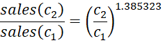
Thus a 10% increase in capital results in a 1.1^1.385323 – 1 = 14.1149% increase in sales. Similarly, a 10% increase in labor costs results in a 10.876% reduction in sales.

Of course, all of this is based on the regression model being valid, which may not be the case, especially since we have not taken unobserved time-invariant effects into account. We now look at the model using differencing.

Example using differencing

As described previously, we need to look at the differences between the two time periods for each of the 8 companies. This is shown on the left side of Figure 2.

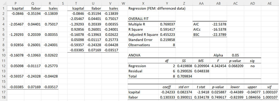
Figure 2 – Regression using differencing

We first place the formula =IF($B2=2012,””,C2-C3) in cell P2 and then highlight the range P2:R16 and press Ctrl-R and Ctrl-D. The result has some blank rows, which can be eliminated by sorting or by placing the Real Statistics array formula =DELROWS(P1:R16,TRUE) in range T1:V9. We can now perform OLS regression using Real Statistics’ Linear Regression data analysis tool to obtain the results shown on the right side of Figure 2.

We now see that labor doesn’t make a significant contribution and in the period 1992 to 1998, increased capital expenditures made a significant, but negative, contribution to sales results, which is counterintuitive but consistent with the data.

Using a dummy time variable

In the differenced model,  we no longer retained any information about the effects for 2010 or 2012, only their differences between the two years. We could, of course, have added the dummy variable yr12_t to the model, where yr12_t = 1 when t = 2012 and yr12_t = 0 when t = 2010. Since yr12_t doesn’t vary based on the firm, it doesn’t take an i subscript.

We can now create the differenced model exactly as done above except that now we have to add the yr12_t variable. Essentially, we can view this model as having two intercepts, b_o when t = 2010 and b₀ + b₁ when t = 2012. Thus

The differenced model is now

which is the same model that we analyzed in Figure 2, except that this time there is an intercept.

Note that we could also add interaction terms such as lcapital_i12⋅yr12_t if it suits our purpose. We could also add dummy variables for the cities in the same manner as we have done for the time periods (see Least-squares Dummy-Variable Model).

Examples Workbook

Click here to download the Excel workbook with the examples described on this webpage.

References

UCLA Statistical Consulting Group (2021) FAQ How do I interpret a regression model when some variables are log transformed?
https://stats.oarc.ucla.edu/other/mult-pkg/faq/general/faqhow-do-i-interpret-a-regression-model-when-some-variables-are-log-transformed/

Gujarati, D. & Porter, D. (2009) Basic econometrics. 5th Ed. McGraw Hill
http://www.uop.edu.pk/ocontents/gujarati_book.pdf

Hill, R. C., Griffiths, W. E., Lim, G. C. (2018) The principles of econometrics. 5^th edition. Wiley.