Overview
Since ANCOVA is essentially regression with some additional assumptions, we can still construct an ANCOVA-like solution using regression even when the homogeneity of slopes assumption is violated, which occurs when there is significant interaction between the covariate and the independent variable.
Example
Example 1: A study was conducted to compare three different teaching methods A, B, and C on the performance of racing drivers factoring out the initial skill levels of the drivers.
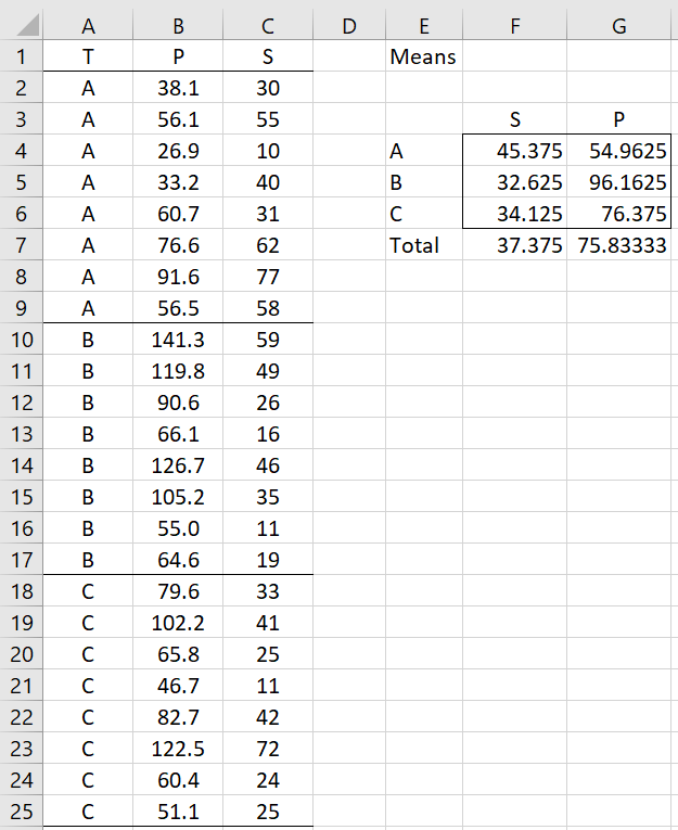
24 drivers were included in the study, with 8 drivers in each of the three treatment groups, as shown in Figure 1.
Figure 1 – Sample data
Here T stands for the treatment group (A, B, or C), S for the skill level, and P for the performance after training. The means of skill and performance for each of the groups as well as the overall means are shown on the right side of the figure.
Chart to check slopes
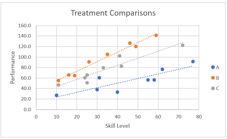
We graph the (S, P) points for each of the three groups and fit a linear trend line for each group using Excel’s Chart capability, as shown in Figure 2.
Figure 2 – Comparison between the three treatments
Regression to check slopes
The slopes of the lines are similar but not exactly the same. To explore this further, we can use regression to check whether there is a significant difference.
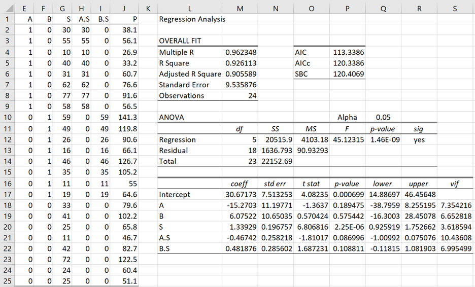
We use the dummy coding where A = 1 if T = A and A = 0 otherwise and B = 1 if T = B and B = 0 otherwise. We also represent the interaction between A and S by A.S and between B and S by B.S. The results of the regression are shown in Figure 3.
Figure 3 – Regression including interactions
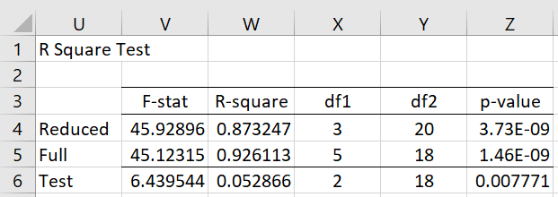
As described in Testing Significance of Extra Variables, we can determine whether the inclusion of the interactions (BS and CS) makes a significant difference in the regression model. As shown in Figure 4, the answer is yes since p-value = .0078.
Figure 4 – Significance test
Row 5 of this figure is derived from the regression in Figure 3. Row 4 is derived from the regression model (not shown) where the X values exclude the A.S and B.S interaction data. The F-statistic in cell V6 is calculated via the formula =W6*Y6/(X6*(1-W5)) while W6 contains =W5-X4, X6 contains =X5-X4 and Y6 contains the formula =Y5. Finally, the p-value in cell Z6 is calculated by the formula =F.DIST.RT(V6,X6,Y6).
Alternatively, the p-value can be calculated by the Real Statistics worksheet formula =RSquareTest(E2:I25,E2:G25,J2:J25).
Details
From Figure 3, setting the values of B and C to 0 or 1 as required, we observe
E[P|T=C, S] = b0+bS S = 30.6173 + 1.3393 S
E[P|T=A, S] = (b0+bA) + (bS + bA.S) S = (30.6173–15.2703) + (1.3393–0.4674) S
E[P|T=B, S] = (b0+bB) + (bS + bB.S)S = (30.6173+6.0752) + (1.3393+0.4819) S
which simplies to
E[P|T=C, S] = 30.6173 + 1.3393 S
E[P|T=A, S] = 15.4014 + 0.8729 S
E[P|T=B, S] = 36.7470 + 1.8212 S
From the above three linear equations, we see that when plotting performance vs. skill level, the slopes of the trendlines for treatments A, B, and C, as shown in Figure 2, are 0.8729, 1.8212, and 1.3393, respectively.
We conclude from the first of the equations that for a person at skill level S = 0, the mean performance after treatment A is 15.4014. Similarly, the mean performance after treatment B for a person with zero skill level is 36.7470 and the mean performance after treatment C for a person with zero skill level is 30.6173.
Since none of the subjects in the experiment have skill level S = 0, it would be better to use a more realistic value for S, such as the mean skill level, which is 37.375 as calculated by =AVERAGE(C2:C25). Using the above formulas, we see that for a person of average skill level, the average performance after treatments A, B, and C are 47.99, 104.81, and 80.73, respectively.
Centering
Actually, if we had subtracted the mean skill value of 37.275 from all the values in column C of Figure 3 (called centering the skill values), we would have obtained the same mean performance values of are 47.99, 104.81 and 80.73 for the three treatments when S is set equal to zero. This can be seen in Figure 5.
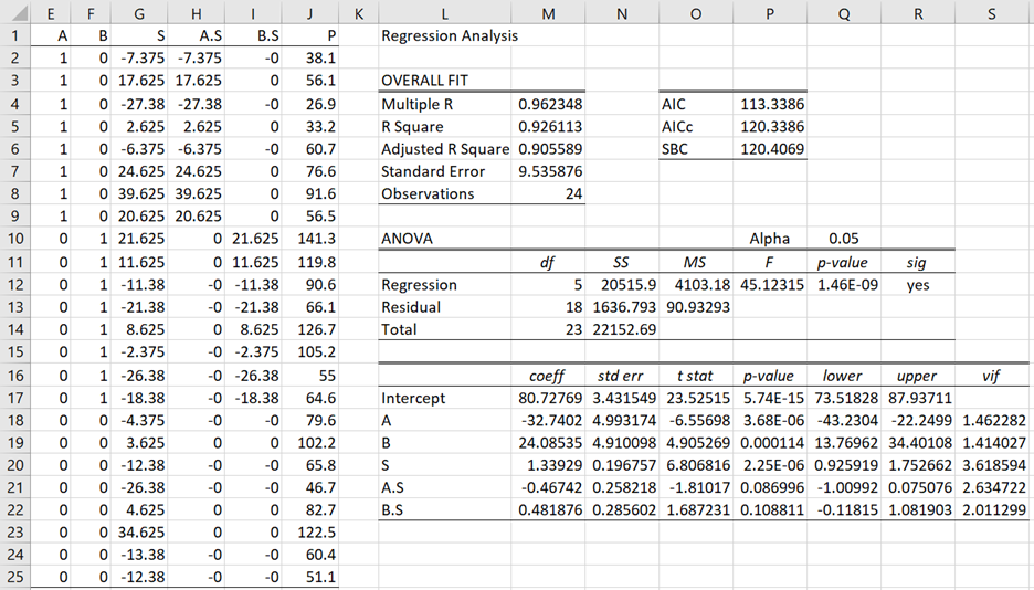
Figure 5 – Regression after centering the skill values
Details
This time, we observe that
E[P|T=C, S] = b0+bS S = 80.7277 + 1.3393 S
E[P|T=A, S] = (b0+bA) + (bS + bA.S) S = (80.7277-32.7402) + (1.3393–0.4674) S
E[P|T=B, S] = (b0+bB) + (bS + bB.S)S = (80.7277+24.0854) + (1.3393+0.4819) S
which simplifies to
E[P|T=C, S] = 80.7277 + 1.3393 S
E[P|T=A, S] = 47.9875 + 0.8729 S
E[P|T=B, S] = 104.813 + 1.8212 S
Since b0 represents the mean performance of subjects that take treatment C when S = 0 and b0 + bA represents the mean performance of subjects that take treatment A when S = 0, then the value bA = -32.7402 represents the increase in performance for subjects with average skill level taking treatment A over those taking treatment C. Similarly, the value bB = 24.0854 represents the increase in performance for subjects with average skill taking treatment B over those taking treatment C. Also, the value bB – bA = 24.0854 – (-32.7402) = 56.8256 represents the increase in performance for subjects with average skill taking treatment B over those taking treatment A.
Conclusions
Since the p-value of b0 is quite small (as seen from cell P18 of Figure 5), we conclude that the mean performance for subjects with average skill level after taking treatment A is significantly different from those taking treatment C. Similarly, based on the p-value in cell P19, we conclude that the mean performance for subjects with average skill level after taking treatment B is significantly different from those taking treatment C. Also since the p-value of b0 is quite small (cell P17), the mean performance of subjects with average skill after taking treatment C is significantly different from zero.
bA.S = -0.467 represents the change in slope for treatment A over C. Since this value is negative, the slope for treatment C is steeper than that for treatment A. bB.S = .4819 represents the change in slope for treatment B over treatment C. Since this value is positive, the slope for treatment B is steeper than that for treatment C.
Once again, we can look at the p-values of bA.S and bB.S to determine whether these differences in slope are significant. From cells P21 and P22 of Figure 5, we conclude that the difference between the slopes of treatments A and C is not significant and the difference between the slopes of B and C is also not significant.
From cell M17, we see that mean performance for subjects with average skill level taking treatment C is 80.7277 and is between 73.52 and 87.94 with 95% confidence. We also see (from cell P20) that for every 10 points extra in skill level, performance for subjects in the C treatment group increases by about 13.4 points. From cell P20, we see that this value is significantly different from zero, and is between 9.3 and 17.5 with 95% confidence.
Examples Workbook
Click here to download the Excel workbook with the examples described on this webpage.
References
Seltman, H. J. (2018) Experimental design and analysis
https://stat.cmu.edu/~hseltman/309/Book/PrefTOC.pdf
PennState (2024) Unequal slopes model: salary example
https://online.stat.psu.edu/stat502/lesson/9/9.5
Thank you for your guidance! Complicated ideas were elaborated clearly.
What are pros and cons of ANCOVA and Regression when we apply them to Quasi-experimental design?
It seems Regression does not require any assumptions check, why do we still have ANCOVA while Regression can help to answer the same inquiry?
Looking forward to hearing from you
Hello Thanh,
1. ANOVA and ANCOVA are both regression in disguise.
2. Regression does have assumptions, but ANCOVA has more assumptions. This webpage shows that you can do “ANCOVA” even when these extra assumptions are not met.
Charles