MA(q) Process Basic Concepts

Introduction

A q-order moving average process, denoted MA(q), takes the form

Thinking of the subscripts i as representing time, we see that the value of y at time i is a linear function of past errors. We assume that the error terms are independently distributed with a normal distribution with mean zero and a constant variance σ². Thus

ε_i ∼ N(0, σ²)          cov(ε_i, ε_j) = 0 if i ≠ j

An MA(q) process can also be expressed as

where z_i = y_i – μ. Thus, we can often simplify our analyses by restricting ourselves to the case where the mean is zero.

Using the lag operator, we can express a zero-mean MA(q) process as

where

Mean and variance

Property 1: The mean of an MA(q) process is μ.

Property 2: The variance of an MA(q) process is

Autocorrelation

Property 3: The autocorrelation function of an MA(1) process is

Property 4: The autocorrelation function of an MA(2) process is

We now generalize these properties to all MA(q).

Property 5: The autocorrelation function of an MA(q) process is

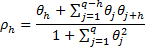
for h ≤ q and ρ_h = 0 for h > q

Observation: The proofs of Property 1 – 5 are given in Moving Average Proofs.

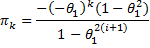
Property 6: The PACF of an MA(1) process is

where 1 ≤ j < n.

If the process is invertible (see Invertible MA(q) Processes), then

MA(1) Example

Example 1: Simulate a sample of size 199 from the MA(1) process y_i = 4 + ε_i + .5ε_i-1 where ε_i ∼ N(0,2).

Thus μ = 4, θ₁ = .5 and σ = 2. We simulate the independent ε_i by using the Excel formula =NORM.INV(RAND(),0,2) in column B of Figure 1 (only the first 20 of 199 values are shown). The y_i values are calculated by placing the formula =4+B5+0.5*B4 in cell C5, highlighting the range C5:C203, and pressing Ctrl-D. The graph of the y values is shown on the right side of Figure 1. As you can see, no particular pattern is visible.

Figure 1 – Simulated MA(1) data

By Properties 1 and 2, the theoretical values for the mean and variance are μ = 4 and var(y_i) = σ²(1+) = 2²(1+.5²) = 5. These compare to the actual time series values of y̅ = AVERAGE(C6:C204) = 4.358 and s² = VAR.P(C6:C204) = 4.401.

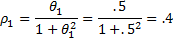
The ACF values are shown for lags 1 through 15 in Figure 2. These are calculated from the y values as in Example 1 of AR(p) Process Basic Concepts. Note that the ACF value at lag 1 is .301285. Based on Property 3, the population ACF value at lag 1 is

MA(1) ACF

The ACF values for lags h > 1 vary from about -.18 to .16, compared to the theoretical value of ρ_h = 0 (per Property 3). As you can see from Figure 2, the sample values can be quite different from the theoretical values.

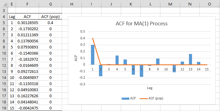
Figure 2 – ACF for MA(1) process

Observation: By Property 3

But note that

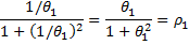
and so the reciprocal of θ₁ yields the same ACF. Thus, if we are seeking a coefficient θ₁ that yields a particular ρ₁ value, we can always choose a coefficient whose absolute value is at most 1. In fact, it turns out that there is always a unique such θ₁ whose absolute value is less than 1.

This is also true for any MA(q) process, and so we will restrict our MA(q) processes to those where |θ_j| < 1 for all j. This also ensures that the MA(q) process is invertible (see Invertible MA(q) Processes).

MA(1) PACF

Example 2: Chart PACF for the data in Example 1.

The approach is as described in Example 1 of Partial Autocorrelation Function. The chart is shown in Figure 3.

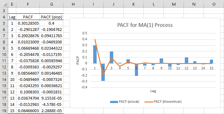
Figure 3 – Graph of PACF for MA(1) Process

The theoretical PACF values are calculated using Property 6. In particular, we insert the following formula in cell G5, highlight the range G5:G19 and press Ctrl-D.

=-((-0.5)^E5*(1-0.5^2)/(1-0.5^(2*E5+2)))

Note that we couldn’t use the following formula

=-(-0.5)^E5*(1-0.5^2)/(1-0.5^(2*E5+2))

This is because Excel incorrectly evaluates any expressions of the form -a^n as if they were (-a)^n. Thus –1^2 and –(–1)^2 are evaluated as 1 instead of -1.

Observation: We can see from Figure 3 that the absolute value of the PACF values tends towards zero as the lag increases. This is generally true for an MA(q) model.

Links

↑ Moving average processes

Examples Workbook

Click here to download the Excel workbook with the examples described on this webpage.

References

Greene, W. H. (2002) Econometric analysis. 5th Ed. Prentice-Hall
https://www.ctanujit.org/uploads/2/5/3/9/25393293/_econometric_analysis_by_greence.pdf

Gujarati, D. & Porter, D. (2009) Basic econometrics. 5th Ed. McGraw Hill
http://www.uop.edu.pk/ocontents/gujarati_book.pdf

Hamilton, J. D. (1994) Time series analysis. Princeton University Press
https://press.princeton.edu/books/hardcover/9780691042893/time-series-analysis

Wooldridge, J. M. (2009) Introductory econometrics, a modern approach. 5th Ed. South-Western, Cegage Learning
https://cbpbu.ac.in/userfiles/file/2020/STUDY_MAT/ECO/2.pdf

Wei, W. (2006) Time series analysis: univariate and multivariate methods, 2nd edition. Pearson Addison Wesley https://www.researchgate.net/publication/236651810_Time_Series_Analysis_Univariate_and_Multivariate_Methods_2nd_edition_2006