Validity of Correlation Matrix and Sample Size

Basic Concepts

Factor analysis doesn’t make sense when there is either too much or too little correlation between the variables. When reducing the number of dimensions we are leveraging the inter-correlations. E.g. if we believe that three variables are correlated to some hidden factor, then these three variables will be correlated to each other. You can test the significance of the correlations, but with such a large sample size, even small correlations will be significant, and so a rule of thumb is to consider eliminating any variable which has many correlations less than 0.3.

Reproduced Correlation Matrix

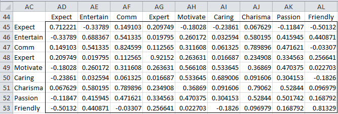
We can calculate the Reproduced Correlation Matrix, which is the correlation matrix of the reduced loading factors matrix.

Figure 1 – Reproduced Correlation Matrix

Referring to Figure 2 of Determining the Number of Factors, the reproduced correlation in Figure 1 is calculated by the array formula

=MMULT(B44:E52,TRANSPOSE(B44:E52))

By comparing the reproduced correlation matrix in Figure 1 to the correlation matrix in Figure 1 of Factor Extraction, we can get an indication of how good the reduced model is. This is what we will do next.

Error Testing

We can also look at the error terms, which as we observed previously, are given by the formula

Our expectation is that cov(e_i, e_j) ≈ cov(ε_i, ε_j) = 0 for all i ≠ j. If too many of these covariances are large (say > .05) then this would be an indication that our model is not as good as we would like.

The error matrix, i.e. R – LL^T, for Example 1 of Factor Extraction is calculated by the array formula,

=B6:J14-MMULT(B44:E52,TRANSPOSE(B44:E52))

(referring to cells shown in Figure 1 of Factor Extraction and Figure 2 of Determining the Number of Factors) and is shown in Figure 2.

Note that the main diagonal of this table consists of the specific variances (see Figure 3 of Determining the Number of Factors), as we should expect. There are quite a few entries off the diagonal that look to be significantly different from zero. This should cause us some concern, perhaps indicating that our sample is too small. One other thing worth noting is that the same error matrix will be produced if we use the original loading factors (from Figure 2 of Determining the Number of Factors) or the loading factors after Varimax rotation (Figure 1 of Rotation).

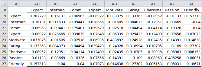
Figure 2 – Error Matrix

Bartlett’s Test

Note too that if overall the variables don’t correlate, signifying that the variables are independent of one another (and so there aren’t related clusters that will correlate with a hidden factor), then the correlation matrix would be approximately an identity matrix. We can test (called Bartlett’s Test) whether a population correlation matrix is approximately an identity matrix using Box’s test.

For Example 1 of Factor Extraction, we get the results shown in Figure 3.

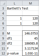
Figure 3 – Bartlett’s Test

We first fill in the range L5:M6. Here cell L5 points to the upper left corner of the correlation matrix (i.e. cell B6 of Figure 1 of Factor Extraction) and cell L6 points to a 9 × 9 identity matrix. 120 in cells M5 and M6 refers to the sample size. We next highlight the 5 × 1 range M8:M12, enter the array formula BOX(L5:M6), and then press Ctrl-Shft-Enter.

Since p-value < α = .001, we conclude there is a significant difference between the correlation matrix and the identity matrix.

Partial Correlation Matrix

Of course, even if Bartlett’s test shows that the correlation matrix isn’t approximately an identity matrix, especially with a large number of variables and a large sample, it is possible for there to be some variables that don’t correlate very well with other variables. We can use the Partial Correlation Matrix and the Kaiser-Meyer-Olkin (KMO) measure of sample adequacy (MSA) for this purpose, described as follows.

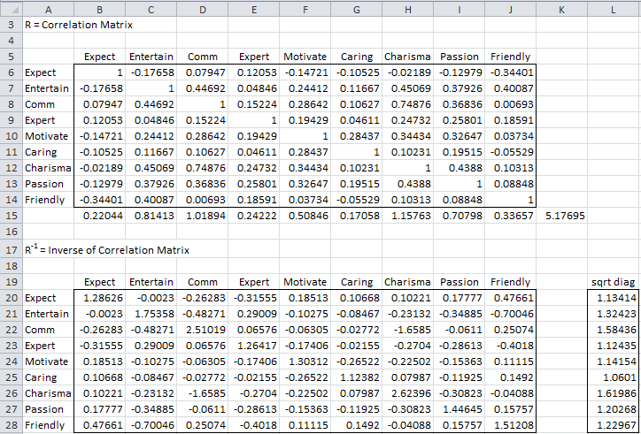
It is not desirable to have two variables that share variance with each other but not with other variables.  As described in Multiple Correlation this can be measured by the partial correlation between these two variables. To calculate the partial correlation matrix for Example 1 of Factor Extraction, first, we find the inverse of the correlation matrix, as shown in Figure 4.

Figure 4 – Inverse of the correlation matrix

Range B6:J14 is a copy of the correlation matrix from Figure 1 of Factor Extraction (onto a different worksheet). Range B20:J28 is the inverse, as calculated by =MINVERSE(B6:J14). We have also shown the square root of the diagonal of this matrix in range L20:L28 as calculated by =SQRT(DIAG(B20:J28)), using the Real Statistics DIAG array function. The partial correlation matrix is now shown in range B33:J41 of Figure 5.

Figure 5 – Partial correlation matrix

The partial correlation between variables x_i and x_j where i ≠ j, keeping all the other variables constant, is given by the formula

where Z = the list of variables x₁, …, x_k excluding x_i and x_j, and the inverse of the correlation matrix is R^-1 = [p_ij]. Thus the partial correlation matrix shown in Figure 5 can be calculated using the array formula

=-B20:J28/MMULT(L20:L28,TRANSPOSE(L20:L28))

Since this formula results in a matrix whose main diagonal consists of minus ones, we use the slightly modified form to keep the main diagonal all ones:

=-B20:J28/MMULT(L20:L28,TRANSPOSE(L20:L28))+2*IDENTITY()

Kaiser-Keyer-Olkin (KMO)

The Kaiser-Meyer-Olkin (KMO) measure of sample adequacy (MSA) for variable x_j is given by the formula

where the correlation matrix is R = [r_ij] and the partial covariance matrix is U = [u_ij]. The overall KMO measure of sample adequacy is given by the above formula taken over all combinations and i ≠ j.

KMO takes values between 0 and 1. A value near 0 indicates that the sum of the partial correlations is large compared to the sum of the correlations. This indicates that the correlations are widespread and so are not clustering among a few variables, which would indicate a problem for factor analysis. On the contrary, a value near 1 indicates a good fit for factor analysis.

For Example 1 of Factor Extraction, values of KMO are given in Figure 6.

Figure 6 – KMO measures of sample adequacy

E.g. the KMO measure of adequacy for Entertainment, KMO₂ (cell C46) is calculated by the formula =C15/(C15+C42) where C15 contains the formula =SUMSQ(C6:C14)-1 (here one is subtracted since we are only interested in the correlations with other variables and not with Entertainment with itself) and C42 contains the formula =SUMSQ(C33:C41)-1. Similarly, the overall KMO (cell K46) is calculated by the formula =K15/(K15+K42), where K15 contains the formula =SUM(B415:J415) and K42 contains the formula =SUM(B42:J42).

Interpreting the KMO

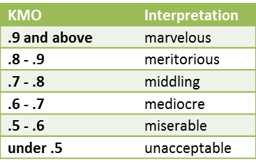
The general rules for interpreting the KMO measures are given in the following table

Figure 7 – Interpretations of KMO measure

As can be seen from Figure 6, the Expectation, Expertise, and Friendly variables all have KMO measures less than .5, and so are good candidates for removal. Such variables should be removed one at a time and the KMO measure recalculated since these measures may change significantly after the removal of a variable.

It should be noted that the matrix all of whose non-diagonal entries are equal to the corresponding entries in the Partial Correlation Matrix and whose main diagonal consists of the KMO measures of the individual variables is known as the Anti-image Correlation Matrix.

Collinearity and Haitovsky’s Test

At the other extreme of testing correlations that are too low is the case where some variables correlate too well with each other. In this case, the correlation matrix approximates a singular matrix, and the mathematical techniques we typically use break down. A correlation coefficient between two variables of more than 0.8 is a cause for concern. Even lower correlation coefficients can be a cause for concern since two variables correlating at 0.9 might be less of a problem than three variables correlating at 0.6.

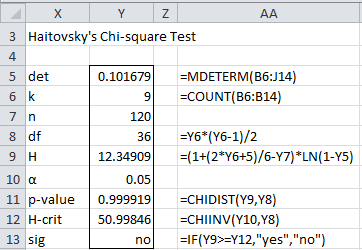
Multicollinearity can be detected by looking at det R where R = the correlation matrix. If R is singular then det R = 0. A simple heuristic is to make sure that det R > 0.00001. Haitovsky’s significance test provides a way for determining whether the determinant of the matrix is zero, namely define H as follows and use the fact that H ~ χ² (m) where

and k = number of variables, n = total sample size and m = k(k – 1)/2.

Figure 8 carries out this test for Example 1 of Factor Extraction.

Figure 8 – Haitovsky’s Test

The result is not significant, and so we may assume that the correlation matrix is invertible.

Sample Size

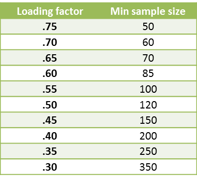
In addition to the KMO measures of sample adequacy, various guidelines have been proposed to determine how big a sample is required to perform exploratory factor analysis. Some have proposed that the sample size should be at least 10 times the number of variables and some even recommend 20 times. For Example 1 of Factor Extraction, a sample size of 120 observations for 9 variables yields a 13:1 ratio. A better indicator of sample size is summarized in the following table:

Figure 9 – Sample size requirements

The table lists the sample size required based on the largest loading factor for each variable. Thus if the largest loading factor for some variable is .45, this would indicate that a sample of at least 150 is needed.

Per [St], a factor is reliable provided

• There are 3 or more variables with loadings of at least .8
• There are 4 or more variables with loadings of .6 or more
• Finally, there are 10 or more variables with loadings of .4 or more and the sample size is at least 150
• Otherwise, a sample of at least 300 is required

References

Haitovsky, Y. (1969) Multicollinearity in regression analysis: a comment. Review of Economics and Statistics, 51 (4), 486-489.
https://www.jstor.org/stable/1926450

Field, A. (2009) Discovering statistics using SPSS (3rd Ed). Sage.
https://www.scirp.org/(S(351jmbntvnsjt1aadkposzje))/reference/ReferencesPapers.aspx?ReferenceID=1866193