Objective
We now show three methods for estimating the coefficients in a multinomial logistic model, namely: (1) using the coefficients described by the multiple binary models, (2) using Solver and (3) using Newton’s method. We explore the first approach here. Click on the above links to explore the other two approaches.
Example
Example 1: A new drug was tested for the treatment of certain types of cancer patients. Figure 1 shows the data for a sample of 860 patients, 449 male (Gender = 0) and 411 women (Gender = 1) given the cancer treatment at various dosages. Three outcomes were measured after 5 years: the patient was cured (i.e. cancer free after 5 years), the patient died or the patient was alive but still had cancer.
Build a multinomial logistic regression model based on this data and use it to predict the probability of the three outcomes for men and women at a dosages of 24 mg and 24.5 mg.
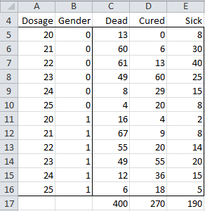
Figure 1 – Data for Multinomial Logistic Regression example
In each case we use Dead as the reference outcome. Generally it is best to use the outcome with the largest sample size (400 for Dead), although the end result will be the same if another choice is made.
The key components of the model are shown in Figure 2.
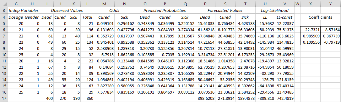
Figure 2 – Multinomial logistic regression model (part 1)
The coefficients are derived from the two binary models: Cured + Dead and Sick + Dead, i.e. the binary logistic regression model based on the data in A5:D16 and the binary logistic regression model based on the data in the range A5:C5 + E5:E16. The fact that the data range for the second model is not contiguous is not a problem since we will be using the Real Statistics MLogitExtract function to extract the correct outcomes from the original data range.
Worksheet Function
Real Statistics Function: The Real Statistics Resource Pack provides the following array function where R1 is a summary data range for multinomial logistic regression with outcomes for the dependent variable of 0, …, r.
MLogitExtract(R1, r, s, head): fill the highlighted range with the columns defined by string s from the data from R1. The string s takes the form of a comma delimited list of numbers 0, …, r. If head = TRUE (default) then R1 includes column headings, while if head = FALSE then R1 does not include column headings. Also, the output will contain column headings if head = TRUE and it will contain only data if head = FALSE.
Example
For the Cured + Dead binary model we use the data range defined by =MLogitExtract(A4:E16,2,”1,0”) or =MLogitExtract(A5:E16,2,”1,0”,False). The first formula includes column headings and the second does not. Here “1,0” means that the data for outcome 1 (column J) is used followed by the data for outcome 0 (column I). The second argument has value 2 since the outcomes are 0, 1, 2. It is important that the reference outcome (i.e. 0) is listed second so that “success” in the binary logistic regression model is for the non-reference outcome.
For the Sick + Dead binary model we use the data range defined by =MLogitExtract(A4:E16,2,”2,0”) or =MLogitExtract(A5:E16,2,”2,0”,False). The first formula includes column headings and the second does not. The output for =MLogitExtract(A4:E16,2,”2,0”) is shown in Figure 3.
Figure 3 – Use of MLogitExtract function
In fact for our purposes here we don’t need to explicitly display the results of the MLogitExtract function. Instead we use the MLogitExtract formula as an argument in the LogitCoeff formula (see Real Statistics Binary Logistic Regression Functions), which calculates the coefficients for binary logistic regression. In particular, we insert the following array formula in range X6:X8 of Figure 1 to calculate the binary logistic regression coefficients for the Cured + Dead model.
=LogitCoeff(MLogitExtract(A5:E16,2,”1,0″,FALSE))
Similarly, we insert the following array formula in range Y6:Y9 of Figure 1 to calculate the binary logistic regression coefficients for the Sick + Dead model.
=LogitCoeff(MLogitExtract(A5:E16,2,”2,0″,FALSE))
The remaining formulas in Figure 1 are calculated as described in Multinomial Logistic Regression Basic Concepts. E.g. the formulas used for the cells in row 5 are as shown in Figure 4.
Figure 4 – Key formulas from Figure 1
In calculating cell V5 we use the fact that n! = Γ(n+1) where Γ is the gamma function (per Property 1c of Gamma Function). Thus ln n! = GAMMALN(n+1).
Significance Testing
The values of LL0, various R-square estimates, as well as the chi-square test for the significance of the multinomial logistic regression model are displayed in Figure 5.
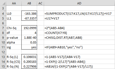
Figure 5 – Multinomial logistic regression model (part 2)
The significance of the two sets of coefficients are displayed in Figure 6.
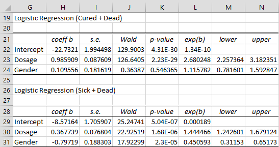
Figure 6 – Multinomial logistic regression model (part 3)
Here the ranges H22:N24 and H29:N31 can be calculated by the array formulas
=LogitCoeff(MLogitExtract(A5:E16,2,”1,0″,FALSE))
=LogitCoeff(MLogitExtract(A5:E16,2,”2,0″,FALSE))
Interpreting the coefficients
That exp(bgender) = 1.116 for Cured + Dead means that for any given dosage women are 11.6% more likely than men to be cured rather than dead. That exp(bgender) = .451 for Sick + Dead means that for any given dosage men are 2.22 (= 1/.451) more likely than women to be sick rather than dead. Since 1.116 – .451 = .665 and 1/.665 = 1.5, for any given dosage men are 50% more likely than women to be cured rather than sick.
That exp(bdosage) = 2.68 for Cured + Dead means one additional mg of medication increases the likelihood of being cured rather than dead 2.68 fold.
Forecasts
Click here for examples of how to obtain forecasts based on the model in Figure 6.
Examples Workbook
Click here to download the Excel workbook with the examples described on this webpage.
References
Wikipedia (2014) Multinomial logistic regression
https://en.wikipedia.org/wiki/Multinomial_logistic_regression
Field, A. (2005) Discovering Statistics Using SPSS. 3rd ed. Sage
https://profandyfield.com/discoverse/dsus/
Cheng, H., (2021) Multinomial logistic regression
https://bookdown.org/chua/ber642_advanced_regression/multinomial-logistic-regression.html
Agresti, A. (2002) Categorical data analysis, Wiley & Sons