Basic Concepts
We now describe how to estimate the parameters of a bivariate normal distribution based on a sample from this distribution, even when some of the data is missing. We use the Expectation-Maximization (EM) algorithm to accomplish this.
In this method, missing data is estimated using an iterative process where each iteration consists of two steps: (1) an M step (maximization) where parameters are calculated based on the missing data results from the previous E step (or via a guess in the initial iteration) and (2) an E step (expectation) where each missing data element is estimated from the parameters in the previous M step.
Missing y values
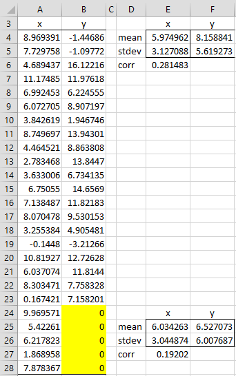
Example 1: Suppose that we have a sample consisting of 25 pairs of the form (x, y) randomly selected from a bivariate normal population, as shown in Figure 1. Note that the y values of the last 5 of the pairs are missing (set to zero in the figure). Estimate the parameters of the bivariate normal distribution.
Figure 1 – Bivariate normal data with missing y values
The mean, standard deviation and correlation coefficient for the completely observed data are shown in range D3:F6 (e.g. cell E4 contains the formula =AVERAGE(A2:A23)), while the same parameters for all 25 sample elements are shown in range D24:F27 where the missing data is arbitrarily filled in with zeros (e.g. cell E25 contains the formula =AVERAGE(A2:A28)). This is the first M step.
Note that we can choose to initialize the missing y values in many different ways (e.g. using the mean of the observed y values).
E and M steps
We now use these parameters to come up with new estimates for the missing values (E step). Here
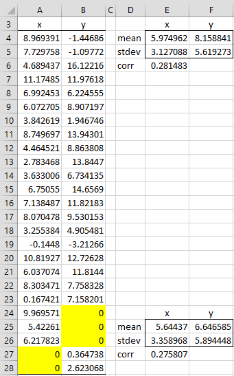
The results are shown on the left side of Figure 2.
Figure 2 – Continuation of EM algorithm
Here, cell I24 contains the formula =F25+E27*F26/E26*(H24-E25), and similarly for the other missing y values (e.g. the same formula is used for cell I25 with H24 replaced by H25 in the formula).
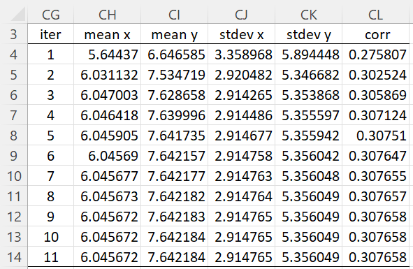
This results in a new set of x and y values in range H2:I28, where the observed values (range H2:I23) are identical to those shown in range A2:B23 of Figure 1. New parameter values in range K24:M27 are now calculated from the complete data in range H2:I28 (the next M step). We continue in this way, as shown on the right side of Figure 2, until we get convergence of the parameter values. These values are shown in Figure 3.
Figure 3 – Convergence Rate
Row 13 (or row 14) contains the estimated parameter values for the original data with 5 missing values.
Missing x and y data
Example 2: Repeat Example 1 for the data in Figure 4. This time, there is both missing x data and y data.
Figure 4 – EM algorithm with missing x and y data
In this case, we calculate missing y values as before and missing x values in a similar way, namely:
The convergence is as shown in Figure 5.
Figure 5 – EM Convergence
Examples Workbook
Click here to download the Excel workbook with the examples described on this webpage.
Links
References
Efron and Hastie (2016) Computer age statistical inference. Cambridge University Press.
Walczak, B., Massart, D. L. (2001) Dealing with missing data: Part II. Chemometrics and Intelligent Laboratory Systems 58 2001. 29–42
https://www.researchgate.net/publication/222039878_Dealing_with_missing_data_Part_II
Mao, L. (2026) The EM: basic theory and practice
https://biostat.wisc.edu/~lmao/missing_data/Chap%202.pdf


