Contingency table missing data | Real Statistics Using Excel

In Independence Testing we show how to test independence using a chi-square test. We now show how to perform such a test when there is missing data (provided the data is missing at random).

Example

Example 1: Impute the missing data in the contingency table shown in Figure 1.

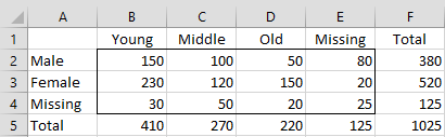
Figure 1 – Contingency Table with missing data

We partition our sample into subsets A, B, and C, in which A consists of those elements where both the row and column components are observed, B consists of those elements where only the row component is observed and C consists of those elements where only the column component is observed. Actually, there is another subset D that consists of those elements where both the row and column component is unobserved (for Example 1 there are 25 such elements, i.e. the value in cell E4). These elements are excluded from the analysis.

The completed contingency table, therefore, contains entries x_ij where

Here $x_{ij}^A$ is observed, but $x_{ij}^B$ and $x_{ij}^C$ are not. The marginal totals are x_i = $\sum{}_{j=1}^c {x_{ij}}$ and x_j = $\sum{}_{i=1}^r {x_{ij}}$ where the completed contingency has r rows and c columns (r = 2 and c = 3 for Example 1).

We also define $x_i^B = \sum{}_{j=1}^c {x_{ij}^B}$ and $x_j^C = \sum{}_{i=1}^r {x_{ij}^C}$ . Note that the values $latex x_{ij}^A$, $x_i^B,$ latex x_j^C$ are observed.

EM Algorithm

Essentially we have a multinomial distribution with parameters p = {p_ij: i ≤ r and j ≤ c}. Our goal is to find the values of p_ij that minimize LL based on the observed data. Initially, we can set p_ij = 1/(rc) (initial M step). The algorithm works as follows:

E step: estimate the values of the based on the observed data and the current estimates of the p_ij (from the previous M step):

M step: estimate the values of the based on the observed data and the current estimates of the x_ij (from the previous E step):

The two steps can be combined so that new values of the p_ij (at step k+1) can be estimated from the previous values of the p_ij (at step k) by

EM Algorithm for Example 1

For Example 1, the analysis begins as shown in Figure 2.

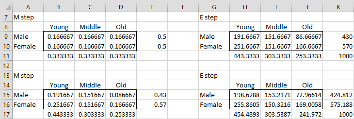
Contingency table initial iterations

Figure 2 – EM algorithm (iterations 1 and 2)

The six cells in range B9:D10 contain the initial M step values of p_ij = 1/6 (for a total of 1). Cell H9 (representing the initial data value x₁₁) contains the worksheet formula =$B$2+$E$2*B9/E9+$B$4*B9/B11 (and similarly for the other cells in range H9:J10, for the first E step). Range B15:D16 contains the array formula =H9:J10/K11 (second M step).

The proceeding E and M steps are calculated in the same way. After 14 steps we arrive at the results shown in Figure 3, demonstrating convergence.

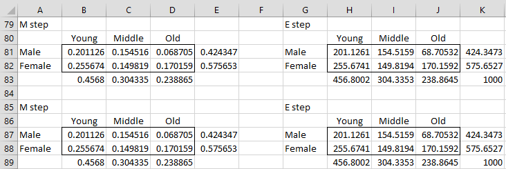
Figure 3 – Convergence of EM algorithm

Thus, we see that we can apportion the missing data as shown in range H81:J82. We can also obtain estimated p_ij values as shown in range B81:D82.

We now calculate the maximum log-likelihood value based on this result. This value is based on the partition consisting of A, B, and C, as follows:

where

We obtain the maximum log-likelihood estimate of -1,559.6, as calculated in Figure 4.

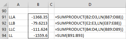
Figure 4 – Maximum log-likelihood estimate

Examples Workbook

Click here to download the Excel workbook with the examples described on this webpage.

Links

↑ EM algorithm

References

Ehlers, R. (2005) Incomplete contingency tables
No longer available online

Howell, D. (2008) The treatment of missing data
https://www.uvm.edu/~statdhtx/StatPages/Missing_Data/MissingDataFinal.pdf

Contingency tables with missing elements