Introduction
Excel provides standard capabilities for sorting and eliminating duplicates. These can be accessed by Data > Sort & Filter|Sort and Data > Data Tools|Remove Duplicates. See Sorting and Filtering for more details.
In Sorting and Filtering Functions, we describe worksheet functions provided in the latest releases of Excel. This webpage describes approaches using Excel formulas that can be employed by all Excel users for sorting.
Also, Real Statistics provides worksheet functions for sorting and elimination of duplicates that are easier to use than the approaches described on this webpage. See Sorting and Removing Duplicates for details.
Sorting numeric data using Excel formulas
We start with sorting numerical data.
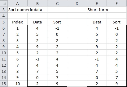
Example 1: Sort the numeric data in column B of Figure 1.
Figure 1 – Sorting numeric data using standard Excel formulas
Create a column of indices in column A by putting 1 in cell A6, the formula =A6+1 in cell A7, and then filling down (by highlighting the range A7:A15 and pressing Ctrl-D). Next place the formula =SMALL(B$6:B$15,A4) in cell C6, highlight the range C6:C15, and press Ctrl-D (to fill down). Column C now contains the same data as in column B but in sorted order.
Sorting is achieved since the formula =SMALL(B$4:B$13, d) has the value of the dth smallest element in the range B6:B15). This approach only works for numeric data. If any of the cells is empty or contains non-numeric data it will not be sorted, but instead the error value #NUM! will appear at the end of the sorted list in column C.
The column of indices (column A) is not really necessary since the same effect can be achieved using the ROW function (see column F of Figure 1). This time we put the formula =SMALL(E$6:E$15,ROW(E6)-ROW(E$6)+1) in cell F6, highlight F6:F15 and press Ctrl-D.
Sorting numeric data w/o duplicates using Excel formulas
Example 2: Sort the data from Example 1 dropping any duplicate entries.
Figure 2 – Sorting without duplicates
Here the data is contained in column I. To eliminate duplicates we need to count the number of times each data item in column I occurs (column J) by placing the formula =COUNTIF(I7:I$16,”=”&I6) in cell J6, highlighting range J6:J15 and pressing Ctrl-D. We now want to retain those elements whose count is 0 in column J. We do this by placing =IF(J6=0,I6,””) in cell K6 and filling down.
Column K now contains the same elements as in column I but without duplicates. We next sort the resulting elements as we did in Example 1. The result is shown in column L. Note that the extra cells are filled with the error code #NUM!. We can combine some of the steps as shown on the right side of Figure 2. We can also remove the #NUM! entries using formulas such as =IF(ISNUMBER(P6),P6,””).
Sorting alphanumeric data using Excel formulas
Examples 3: Sort the alphanumeric data in column B of Figure 3.
Figure 3 – Sorting alphanumeric data using Excel formulas
The approach used in Example 1 doesn’t work with non-numeric data. This time we need to use the COUNTIF, MATCH, and INDEX functions to accomplish our goal (see Built-in Excel Functions). We rank each of the elements in column B from lowest in alphabetic order to highest in column C: e.g. cell C21 contains the formula =COUNTIF(B$21:B$30,”<“&B21). Note that duplicate entries for ape have the same rank (namely 0) and similarly the duplicate entries for dog and lion have the same ranking (4 and 7 respectively).
We next count the number of occurrences of each word in the list (column D): e.g. cell D21 contains the formula =COUNTIF(B$21:B21,B21). We add these count values from column D to the rank values from column C to obtain a revised ranking in column E. Note that all the elements in the list now have a different ranking and the blank entry has a rank of 0.
Using RANK, MATCH and INDEX
For each data element (from column B) we need to determine its rank (from column E) and put the index of that element (from column A) in the row of E with that rank. E.g. since the index of the first occurrence of lion (namely 1) has rank 8 we put a 1 in the 8th position of column F (i.e. cell F28). This is accomplished using the MATCH function: e.g. cell F21 contains the formula =MATCH(A21,E$21:E$30,0).
Finally, we use the INDEX function to list the data elements in sorted order: e.g. cell G21 contains the formula =INDEX(B$21:B$30,F21). Note that the empty entry is replaced by the error code #N/A placed at the bottom of the list. As in Example 1 we can replace these error codes by a blank (or anything else).
Sorting alphanumeric data w/o duplicates using Excel formulas
Example 4: Sort the data from Example 3 dropping any duplicate entries.
Figure 4 – Sorting alphanumeric data without duplicates
We worked hard to sort repeated elements in Example 3. This time we want to drop these elements. The trick this time is to get the resulting blanks to move to the bottom of the list (as #N/A or blanks). The required formulas for the first row are shown in Figure 5.

Figure 5 – Sample formulas from Figure 4
Note that the revised ranking in column E is required to get the blank entries to occur at the bottom of the list.
Examples Workbook
Click here to download the Excel workbook with the examples described on this webpage.
References
Mellor, L. (2020) Sort and filter using dynamic array functions in Microsoft Excel
https://www.laramellortraining.co.uk/how-to-sort-and-filter-using-dynamic-array-functions-in-microsoft-excel
Stack Overflow (2021) Sortby function combined with Unique combined with filter functions
https://stackoverflow.com/questions/68246608/sortby-function-combined-with-unique-and-filter-functions-how-to-use-it-correcl


