Kaplan-Meier Theory

Property A: For a random variable x, the variance of g(x) can be approximated by

Proof: The proof uses the Delta method; namely, from the Taylor series for any constant a, we have

Thus

Now, let a = the mean of x. Then

Thus

since var(y+c) = var(y), var(c) = 0, and var(cy) = c² ⋅ var(y) for any y and constant c (by Property 3 of Expectation).

Property 1 (Greenwood): The standard error of S(t) for any time t,  t_k ≤ t < t_k+1 is approximately

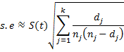
Proof: First we note that

where p_j = 1 − d_j/n_j is the probability that a subject survives to just before t_j. Taking the natural logs

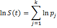Thus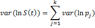

We now assume that the number of subjects that survive in the interval [t_j, t_j+1) has a binomial distribution B(n_j, π_j) where p_j is an estimate for π_j. Since the observed number of subjects that survive in the interval is n_j − d_j, it follows (based on the variance of a binomial random variable) that

Thus

Based on Property A

Thus

But using Property A again, we also have

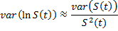
and so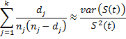

which means that

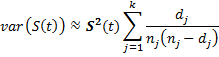
Taking the square root of both sides of the equation completes the proof.

Property 2: The approximate 1−α confidence interval for S(t) for t,  t_k ≤ t < t_k+1, is given by the formula

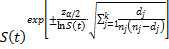
where z_α/2 = NORM.S.INV(1−α/2).

Proof: We could use a confidence interval of S(t) ± z_α/2 ⋅ s.e., but it has the defect that it can result in values outside the range of S(t), namely 0 to 1. Thus it is better to use a transformation that transforms S(t) to the range (-∞,∞) and then take the inverse transformation. We use the transformation ln(−lnx) to accomplish this. This transformation is defined for x = S(t), except when S(t) = 0 or 1.

By Property A

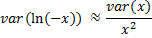
From this and the proof of Property 1, it follows that

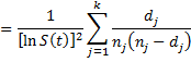
Thus the standard error of ln(-ln S(t))  is

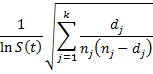
The result now follows by taking the inverse transformations.

Property B: 

Proof: By definition

ThusLinks

↑ Kaplan-Meier