Confidence Ellipse

In the case of a bivariate normal distribution, we can create a plot of the confidence ellipse.

Example

Example 1: Create a chart of the 95% confidence ellipse for the data in range A3:B13 of Figure 1.

We begin by showing how to manually create a confidence ellipse when chi-square = 2.25 (cell H8), which is the same as a 67.5% confidence ellipse, as shown in cell H9 which contains the formula =CHISQ.DIST(H8,2,TRUE).

To create a 95% confidence ellipse, we instead place .95 in cell H9 and the formula =CHISQ.INV(H9,2) in cell H8 (resulting in a chi-square value of 5.99).

Figure 1 – Confidence ellipse (part 1)

Set-up

The covariance matrix for the input data is calculated by the formula =COV(A4:B13), as shown in range D4:E5, with the inverse shown in range D11:E12 as calculated by =MINVERSE(D4:E5). The mean vector is shown in the range D8:E8 where D8 contains the formula =AVERAGE(A4:A13) and E8 contains =AVERAGE(B4:B13).

The eigenvalues of the covariance matrix (range G4:H4) can be calculated using the array formula =eVALUES(D4:E5). Alternatively, for a 2 × 2 matrix, they can be calculated using the fact that the sum of the eigenvalues is equal to the trace of the covariance matrix (=D4+E5) and the product of the eigenvalues is equal to the determinant of the matrix (=D4*E5-E4^2). Solving these two simultaneous equations yields the eigenvalues as shown in cells H13 and H14, as calculated by =(H11+SQRT(H11^2-4*H12))/2 and =H11-H13.

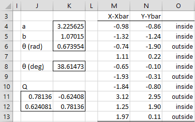
Figure 2 – Confidence ellipse (part 2)

The lengths of the two axes of the ellipse are shown in cells K4 and K5, as calculated by the worksheet formulas =SQRT(G4)*SQRT(H8) and =SQRT(H4)*SQRT(H8). The angle (in radians) the ellipse makes with the x-axis is as shown in cell K6, as calculated by the formula =ATAN2(E4,G4-D4). The angle in degrees is shown in cell K8 using the formula =K6*180/PI(). The rotation Q matrix in range J11:K12 is calculated by the formula =COS(K6) in cells J11 and K12, =SIN(K6) in cell J13, and =-J13 in cell K11.

Column O shows whether each of the data points (in A4:B13) is located inside or outside the ellipse. E.g. the first data point is inside the ellipse (cell O4), This is determined by the following formula:

=IF((D$11*M4+E$11*N4)*M4+(D$12*M4+E$12*N4)*N4>=H$8,”outside”,”inside”)

where cell M4 contains the formula =A4-D$8 and cell N4 contains the formula =B4-E$8.

Creating the Chart

We now create a chart of the ellipse using a scatter chart of points at regular intervals around the ellipse, as shown in Figure 3.

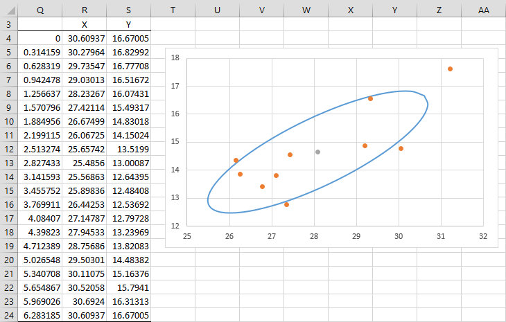
Figure 3 – Confidence ellipse (part 3)

First, we create column Q by placing zero in cell Q4, the formula =PI()/10 in cell Q5 and =Q5+Q$5 in cell Q6. We then highlight range Q6:Q24 and press Ctrl-D. The result is that column Q contains the values 0 to 2π in increments of π/10. Each value in column Q corresponds to a point on the ellipse as shown in columns R and S. E.g. the first such point (shown in cells R4 and S4) is calculated by the formulas

=(J$11*K$4*COS(Q4)+K$11*K$5*SIN(Q4))+D$8

=(J$12*K$4*COS(Q4)+K$12*K$5*SIN(Q4))+E$8

We now highlight the range R4:S24 and select Insert > Charts > Scatter. This creates the chart of the ellipse shown in Figure 3, except that the points are not yet connected. We next click on the chart and select Design > Data|Select Data which brings up the dialog box shown in Figure 4.

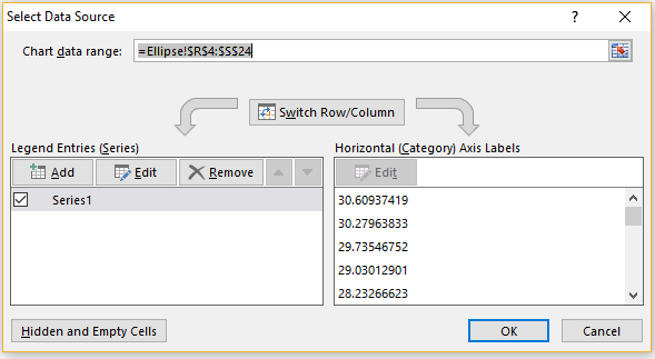
Figure 4 – Select Data Source dialog box

We next click on the Add button and fill in the dialog box that appears as shown in Figure 5, and then click on the OK button.

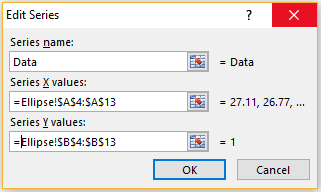
Figure 5 – Add original data points

This adds the original data points to the chart. In a similar fashion, we add the center of the ellipse by again clicking on the Add button in Figure 4 and when the dialog box in Figure 5 appears, insert D8 in the Series X values field and E8 in the Series Y values field.

Connecting the Points

We now need to connect the points in the scatter chart of the ellipse. This is done by clicking on any of the points on the ellipse and selecting Design > Type|Change Chart Type which brings up the dialog box shown in Figure 6.

Figure 6 – Change Chart Type

In the pulldown menu for Series1 (which represents the ellipse) choose the Scatter with Smooth Lines (instead of the Scatter) option.

Increasing the Size of the Chart

As can be seen from Figure 6, the ellipse only occupies a very small portion of the chart. We can fix this using standard Excel chart capabilities, but it is easier to do this using a Real Statistics capability. First, click on the chart and then press Ctrl-m and choose the Change Chart Axes Min/Max data analysis tool. Fill in the dialog box that appears as shown in Figure 7.

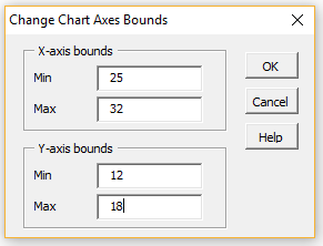
Figure 7 – Change Chart Axes Min/Max dialog box

The result is the chart shown in Figure 3. Note that 4 of the data points are located outside the ellipse, which agrees with the results shown in Figure 2.

Real Statistics Support

See Real Statistics Tool to Create a Confidence Ellipse.

Examples Workbook

Click here to download the Excel workbook with the examples described on this webpage.

Reference

Johnson, R. A., Wichern, D. W. (2007) Applied multivariate statistical analysis. 6th ed. Pearson Prentice-Hall
https://www.webpages.uidaho.edu/~stevel/519/Applied%20Multivariate%20Statistical%20Analysis%20by%20Johnson%20and%20Wichern.pdf