Overview
On this webpage, we describe Real Statistic support for Principal Component Analysis. We illustrate these capabilities using Example 1 from that webpage. The first 10 of 120 data rows for that example are repeated in Figure 1.
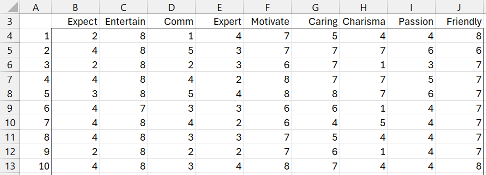
Figure 1 – Dataset
Data Analysis Tool
Starting with Rel 9.8. Real Statistics provides the Principal Component Analysis data analysis tool. To use this tool for Example 1, press Ctrl-m and select the Principal Component Analysis option from the Multivar tab. Next, fill in the dialog box that appears, as shown in Figure 2.
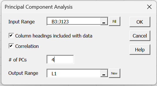
Figure 2 – PCA dialog box
Of course, you won’t know in advance what value to choose for the # of PCs field, but from the scree plot shown below, 4 is a reasonable choice.
After clicking on the OK button, the output shown in Figures 3-6 appears.
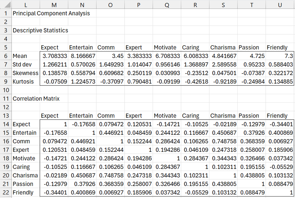
Figure 3 – PCA output (part 1)
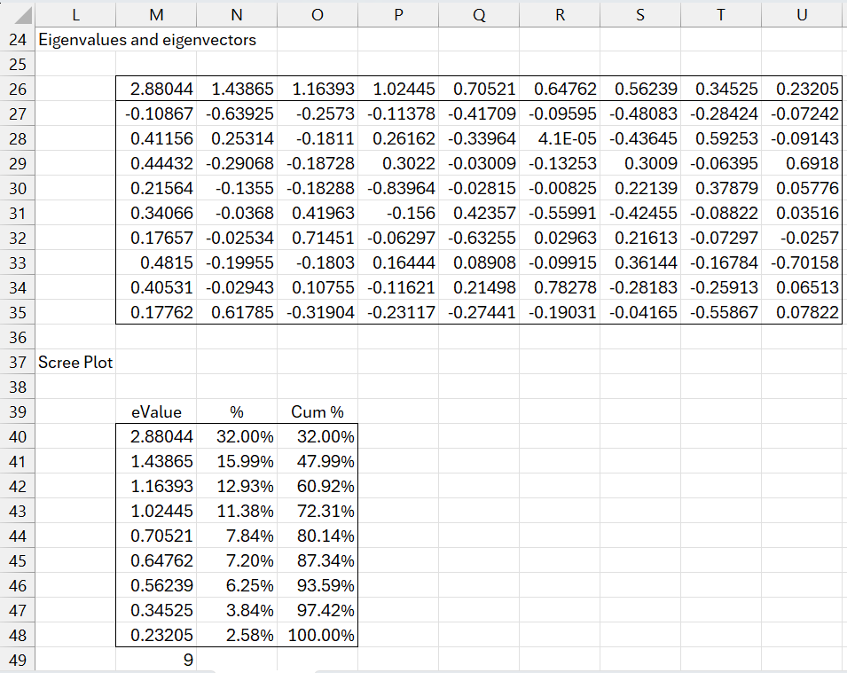
Figure 4 – PCA output (part 2)
Using the table in Figure 4, the data analysis tool outputs the scree plot shown in Figure 5.

Figure 5 – PCA output (part 3)
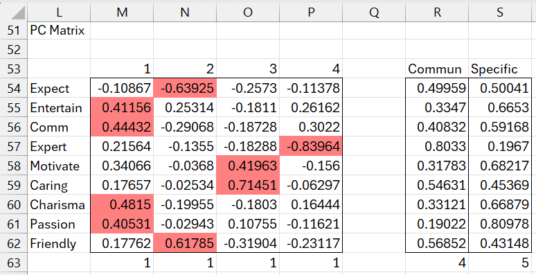
Figure 6 – PCA output (part 4)
Interpretation
The highlighted cells in Figure 6 contain values whose absolute value exceeds .4. The Communalities and Specific columns in Figure 6 are most applicable to Factor Analysis, and are explained in Determining the Number of Factors. The values in range M63:P63 contain the sum of squares of the entries in the corresponding columns, namely 1.
Note that the Entertain, Comm, Charisma, and Passion have a large correlation with PC1. We might, therefore, view PC1 as representing Personality.
Friendly has a large positive association with PC2, while Expectation has a large negative association with PC2. Perhaps we can interpret PC2 as Easy Going.
Motivation and Caring have a positive association with PC3. A possible interpretation, therefore, for PC3 is Supportive.
Finally, as explained in Determining the Number of Factors, we can flip the signs of the entries for PC4, resulting in a positive association between Expertise and PC4. Thus, Expertise is a reasonable interpretation of PC4.
Worksheet Functions
The Real Statistics Resource Pack furnishes the following two worksheet functions.
PCFull(R1, cor): returns the eigenvalues/vectors for the data in R1 (without column headings) based on the correlation matrix when cor = TRUE (default) and the covariance matrix when cor = FALSE
PCScore(R1, nPCs, brev, cor): returns the score matrix for the data in R1 (without column headings) based on nPCs principal components. If nPCs = 0 (default), then nPCs is set to the # of columns in R1. If brev = TRUE (default), then the scores are based directly on the principal components. While, if brev = FALSE, then the scores are translated back into the original data units.
Examples
For our example, =PCFull(B4:J123) returns the results shown in Figure 7. Note that the first row contains the eigenvalues for all 9 principal components, while the next 9 rows contain the corresponding unit eigenvectors. Note that these values are the same as those shown in Figure 4. The final two rows should contain values close to zero, as explained in Eigenvalue/vector Functions.
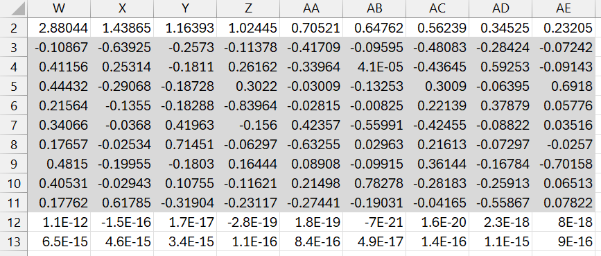
Figure 7 – PCFull output
The formula =PCScore(B4:J123,4) in range AG2:AJ121 of Figure 8 converts the standardized versions of the original data to the equivalent data based on the principal components from Figure 6 (or the first four columns from Figure 7). The figure only displays the first 10 of 120 rows.
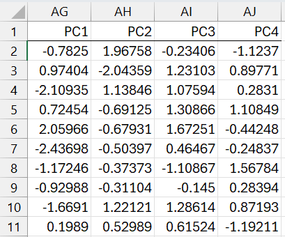
Figure 8 – PCScore output (part 1)
As we explain in Principal Component Analysis, we can now convert these scores back into the original units. This is done using the formula =PCScore(B4:J123,4,FALSE) in range AL2:AT121). The first 10 rows of the output are shown in Figure 9.
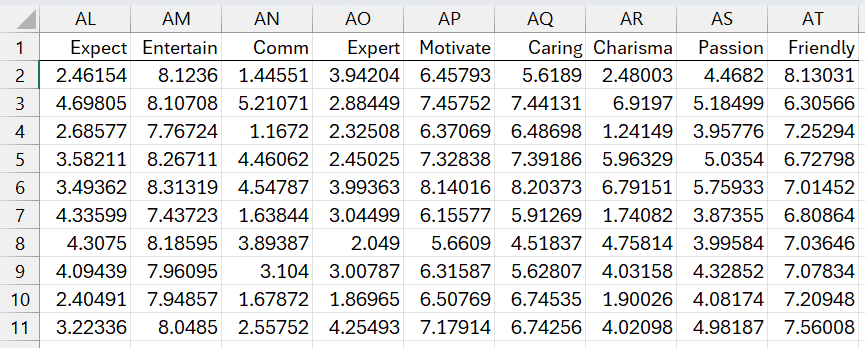
Figure 9 – PCScore output (part 2)
Note that these values are similar to the data values in Figure 1 and represent how much is lost by using only the first 4 PCs instead of all 9. In fact, if all 9 PCs were used, then the output would be identical to the original data.
Using the covariance matrix
You can perform the same analysis using the covariance matrix instead of the correlation matrix. This has the downside that variables with larger unit values will distort the analysis. When the covariance matrix is used, the PCScore function doesn’t need to standardize or unstandardize the data.
Links
↑ Principal component analysis
Examples Workbook
Click here to download the Excel workbook with the examples described on this webpage.
References
Penn State University (2013) STAT 505: Applied multivariate statistical analysis (course notes)
https://online.stat.psu.edu/stat505/Lesson11
Rencher, A.C. (2002) Methods of multivariate analysis (2nd Ed). Wiley-Interscience, New York.
http://math.bme.hu/~csicsman/oktatas/statprog/gyak/SAS/eng/Statistics%20eBook%20-%20Methods%20of%20Multivariate%20Analysis%20-%202nd%20Ed%20Wiley%202002%20-%20(By%20Laxxuss).pdf
Johnson, R. A. and Wichern, D. W. (2007) Applied multivariate statistical analysis. 6th Ed. Pearson.
https://mathematics.foi.hr/Applied%20Multivariate%20Statistical%20Analysis%20by%20Johnson%20and%20Wichern.pdf
Pituch, K. A. and Stevens, J. P. (2016) Applied multivariate statistical analysis for the social sciences. Routledge.
Minitab (2026) Example of principal components analysis
https://support.minitab.com/en-us/minitab/help-and-how-to/statistical-modeling/multivariate/how-to/principal-components/before-you-start/example/