Bootstrapping for Regression | Real Statistics Using Excel

Objective

Our objective is to show how to use bootstrapping in regression modelling. In particular, we describe how to estimate standard errors and confidence intervals for regression coefficients, and prediction intervals for modeled data. Bootstrapping is especially useful when the normality and/or homogeneity of variance assumptions are violated.

See the following links for further information about bootstrapping:

Click here for a description of Excel worksheet functions provided by the Real Statistics Resource Pack in support of bootstrapping for regression models. Eamples are also provided.

Bootstrapping for regression coefficient covariance matrix

We provide two approaches for calculating the covariance matrix of the regression coefficients.

Approach 1 (resampling cases)

We assume that X is fixed. Using the original X, y data, estimate the regression coefficients via

B = (X^TX)^-1X^TY

Next calculate

E = Y – XB

We now create N bootstrap iterations. For each iteration, create an E* by randomly selecting n rows from E with replacement. Next calculate

Y* = XB + E*

and use regression to calculate the regression coefficients B* based on the data in X, Y*. Thus

B* = (X^TX)^-1X^TY*

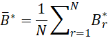
We now calculate the average of these N bootstrap B* values.

Next, we calculate the k × k bootstrap covariance matrix as follows

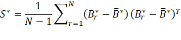
The square roots of the values on the main diagonal of S* serve as the standard errors of the regression coefficients in B.

Approach 2 (resampling residuals)

This time we create N bootstrap iterations as follows. For each iteration, randomly select n random numbers from the set 1, …, n. We now define X* and Y* as follows. For each such random number i assign the ith row of X to the next row in X* and the ith row of Y to the next row in Y*. For this X*, Y*, perform regression to estimate the regression coefficient matrix B*. Now calculate S* as described above to obtain the covariance matrix and standard errors of the regression coefficients.

Bootstrapping regression coefficient confidence intervals

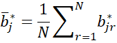
We can use the same two approaches to create confidence intervals for the individual regression coefficients. Using either approach, calculate the N bootstrap k × 1 coefficient matrices B* = [b*_j]. The bootstrap standard error for each element β_j in β can be estimated by

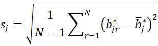
where

We can also calculate a 1 – α confidence interval for each β_j by first arranging the jth coefficient for each bootstrap coefficient matrix in order

The 1 – α confidence interval is then

Bootstrapping confidence intervals for data

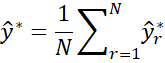
The standard error and confidence interval for ŷ = X₀β where X₀ is a 1 × k+1 row vector (with initial element 1), is produced by first generating N bootstrap values B^*₁, …, B^*_N for the coefficient matrix as described above. For each B^*_r we calculate the predicted value of y for X₀, namely

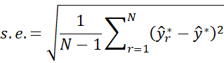
We next take the average of these values

The standard error is then

Arranging the N bootstrapped predicted y values in order

we obtain a 1 – α confidence interval as follows:

Bootstrapping prediction intervals for data

Our goal is to find bounds for y = X₀β + ε. There are two sources of uncertainty: estimate of β by B, and the uncertainty of ε. We use the same as for the confidence interval, except that we need to add uncertainty for ε.

If the homogeneity of variances assumption is met, then for each bootstrap B^*_r we can select one of the n entries in E^*_r at random (call it e^*_r) and use it to serve as the bootstrap version of ε. Here E^*_r = Y^*_r – B^*_rX when using Approach 1 and E^*_r = Y^*_r – B^*_rX^*_rwhen using Approach 2.

This results in a bootstrap y value of

Arranging these in increasing order, we obtain the 1-α prediction interval.

Modification

Instead of using the ordinary residuals, we could use mean-centered variance adjusted residuals. E.g. if E = [e_i] is an n × 1 array of residuals, then the variance adjusted residuals are

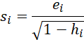
where h_i is the leverage for observation i. (see Regression Residuals). We then find the mean of these values, s, and use the values s_i – s instead of the e_i.

Assumptions

Both the resampling cases and resampling residuals assume that the errors are independent, and so is most relevant for heterogenous error variances.

The resampling residuals also assumes additivity/linearity and homoscedasticity.

In general, the resampling residuals produces tighter, more accurate confidence intervals.

References

Eck, D. J. (2017) Bootstrapping for multivariate linear regression models
https://arxiv.org/abs/1704.07040

Stine, R. A. (1985) Bootstrap prediction intervals for regression
https://www.jstor.org/stable/2288570?seq=1

Fox, J. (2015) Bootstrapping regression models.
Applied Regression Analysis and Generalized Linear Models, 3^rd ed. Sage Publishing
https://us.sagepub.com/sites/default/files/upm-binaries/21122_Chapter_21.pdf

Stack Exchange (2021) Bootstrap prediction interval
https://stats.stackexchange.com/questions/226565/bootstrap-prediction-interval

Roustant, O. (2017) Bootstrap & confidence/prediction intervals
https://olivier-roustant.fr/wp-content/uploads/2018/09/bootstrap_conf_and_pred_intervals.pdf

Bootstrapping Regression Models