Schur’s Factorization

Introduction

In QR Factorization, we show how to construct a QR factorization for any invertible square matrix A (with real elements). In fact, we can use the QR Factorization option of the Matrix data analysis tool to calculate the orthonormal matrix Q and the upper triangular matrix R such that A = QR.

We also show how to use this QR Factorization to calculate the eigenvalues/vectors of a symmetric square matrix. In fact, we can use the Eigenvalues/vectors option of the Matrix data analysis tool (or the functions eigVALSym and eigVECTSym) to calculate the eigenvalues/vectors.

It turns out that the algorithm described can be used to calculate any real-valued eigenvalues even for non-symmetric matrices, but while the eigenvector for the dominant eigenvalue is correct, the other eigenvectors generated aren’t necessarily correct for non-symmetric matrices. One way to find the correct eigenvectors is to use Schur’s factorization.

Basic Concepts

Definition 1: A Schur’s factorization (or Schur’s decomposition) of a square matrix A consists of an orthogonal matrix Q and an upper triangular matrix T such that A = QTQ^T.

Observation: Since by Property 6a of Orthogonal Vectors and Matrices, for an orthogonal matrix Q^-1 = Q^T, it follows from Property 9 of Eigenvalues and Eigenvectors that A and T have the same eigenvalues. But by Property 1d of Eigenvalues and Eigenvectors, the eigenvalues of T are the elements on the main diagonal. Thus, the eigenvalues of A are the elements on the main diagonal of T as well.

Also, since Q^-1 = Q^T, we know that A = QTQ^T is equivalent to T = A^TTA.

Property 1 (Schur’s Factorization): For any n × n invertible matrix A, we can construct a Schur’s factorization.

Proof: The proof is by induction on n. If n = 1, then if A = [a] then A = QTQ^T where Q = [1] and T = [a]. We now assume that the property holds for n and show how to construct a Schur’s factorization for the n+1 × n+1 matrix A.

Let λ be any real eigenvalue of A with corresponding real eigenvector X. These can be found using the QR factorization procedure of Definition 3 of QR Factorization. As usual, we can assume that ||X|| = 1. By Theorem 1 of Orthogonal Vectors and Matrices (Gram-Schmidt), we can construct an n+1 × n+1 orthogonal matrix P whose first column is X. Alternatively, we can construct P using QR Factorization as follows.

In fact, let B = [X E₁ E₂ … E_n] where E_i is a column vector all of whose elements are 0 except for the element in the ith row which is 1 (although if x_n+1 = 0, where x_n+1 is the n+1^th element in X, then replace E_i in the definition of B by E_n+1 for any i such that x_i ≠ 0; such an element exists since X ≠ O). Using Property 6 (QR Factorization), we can construct an orthogonal matrix P and upper triangular matrix R such that B = PR, where the first column of P  is X, and so P = [X C] for some n+1 × n matrix C.

Now since X^TAX = X^TλX = λX^TX = λ and C^TAX = C^TλX = λC^TX = λO = O, we have

where

By the induction hypothesis, there is an orthogonal matrix and upper triangular matrix  such that

Thus

Now define

Then T is upper triangular and Q is orthogonal. Furthermore

Observation: Note that the factorization is not unique. In particular, changing the order of the diagonal elements changes the factorization.

Example

Example 1: Find the Schur’s Factorization for matrix A in range A2:C4 of Figure 1.

We highlight the range A7:C12 and enter the array formula =eVECTOR(A2:C4,500). The eigenvalues of A are found in range A7:C7, namely -4.11718, 2.485349, and -1.36817. Since range A11:C11 contains values of det(A−λI) close to zero, these values are true eigenvalues.

The unit eigenvector corresponding to the first eigenvalue is found in range A8:A10. Since the value in cell A12 is close to zero, this eigenvector is correct. This eigenvector is also entered in range E7:E9 to build the first B matrix (range E7:G9). Note that since the values in cells B12 and C12 are not close to zero, the vectors in B8:B10 and C8:C10 are not eigenvectors.

We now use the array formula =QRFactor(E7:G9) to calculate the P matrix (range E12:G14). Next we use the array formula

=MMULT(TRANSPOSE(E12:G14),MMULT(E2:G4,E12:G14))

to calculate P^TAP (range E17:G19).

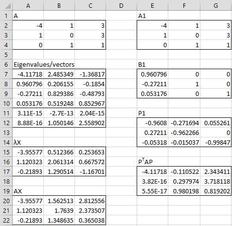
Figure 1 – Schur’s Factorization (step 1)

We now repeat the above procedure on the 2 × 2 matrix A₂ which is formed from the lower right portion (i.e. range F18:G19) of P^TAP, which is repeated in range I2:J3 in Figure 2.

We use the formula =eVECTORS(I2:J3) to obtain the eigenvalues in range I6:J6 and potential eigenvectors in I7:I8 and J7:J8. Once again the first eigenvector is valid (cell I10 is near zero) and the second is not a valid eigenvector (cell J10 is not near zero). The 2 × 2 version of matrix B is shown in range L6:M7 and the corresponding matrix P is shown in range L10:M11 using the formula =QRFactor(L6:M7).

Figure 2 – Schur’s Factorization (step 2)

For any 2 × 2 matrix A, the P matrix is the Q matrix in Schur’s factorization of A. Thus the matrix in range L10:M11 is the Q matrix in Schur’s factorization of the matrix in range L2:M3. To calculate the corresponding T matrix, we first need to calculate P^TAP (range L14:M15) via the array formula

=MMULT(TRANSPOSE(L10:M11),MMULT(L2:M3,L10:M11)).

The four cells in T (range L18:M19) are calculated as follows: =I6 in cell L18, 0 in cell L19, =M14 in cell M18, and =J6 in cell M19.

We now need to calculate the Q and T matrices for the original 3 × 3 matrix A in range A2:C4 of Figure 1. This is shown in Figure 3.

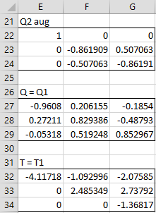
Figure 3 – Schur’s factorization (step 3)

We augment the Q₂ matrix (range L10:M11) from Schur’s factorization of A₂ as shown in range E22:G24, by placing zeros in the first row and column except for a 1 in the first cell and then Q₂ in the lower right portion of the matrix. The Q matrix in Schur’s factorization of our original matrix A is then calculated using the array formula =MMULT(E12:G14,E22:G24), as shown in range E27:G29.

The T matrix in Schur’s factorization is shown in range E32:G34. Here cell E32 contains the formula =A7, cells E33 and E34 contain zeros, range F32:G32 contains the array formula =MMULT(F17:G17,L22:M23) and range F33:G34 contains the array formula =L26:M27. We can also calculate the value of T by the formula

=MMULT(TRANSPOSE(E27:G29),MMULT(E2:G4,E27:G29))

We see that T is an upper triangular matrix and

Q^TQ = MMULT(TRANSPOSE(E27:G29),E27:G29)

is an identity matrix, thus proving that Q is orthogonal. Finally, we see that we can calculate QTQ^T by

=MMULT(E27:G29,MMULT(E32:G34,TRANSPOSE(E27:G29))) 

Worksheet Functions

Real Statistics Functions: The Real Statistics Resource Pack contains the following array functions to calculate Schur’s factorization for matrix A in range R1:

SCHUR(R1, iter, order): returns matrices Q and T such that A = QTQ^T is Schur’s factorization of A. If R1 is an n × n range, the output is a 2n × n range with matrix Q over T.

SCHURQ(R1, iter, order): returns only matrix Q of Schur’s factorization of A

The algorithm used is iterative with iter iterations (default 100). The diagonal of T contains the eigenvalues of A. If order = TRUE or -1 (default) then the eigenvalues are arranged in descending order based on their absolute values. If order = FALSE or 0 then the eigenvalues are in descending order. Finally, if order = +1 then the eigenvalues are not sorted at all.

Data Analysis Tool

Real Statistics Data Analysis Tool: The Schur’s factorization can also be created by using the Schur’s Factorization option of the Matrix data analysis tool.

References

Golub, G. H., Van Loan, C. F. (1996) Matrix computations. 3rd ed. Johns Hopkins University Press
Searle, S. R. (1982) Matrix algebra useful for statistics. Wiley
Perry, W. L. (1988) Elementary linear algebra. McGraw-Hill
Fasshauer, G. (2015) Linear algebra.
https://math.iit.edu/~fass/532_handouts.html
Lambers, J. (2010) Numerical linear algebra
https://www.yumpu.com/en/document/view/41276350