Basic Concepts
We can calculate the confidence interval of a fitted distribution parameter using bootstrapping like that used to calculate the standard error (see Fitted Parameters Standard Error). For any parameter, suppose that β-hat is the fitted estimate of the true parameter value β, and suppose further that the distribution of β – β-hat were known. Then for any α, with 0 < α < 1, there would exist δ1 and δ2 such that

in which case
 and so

yielding a 1–α confidence interval for β of
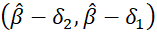
Since β is not known, we estimate it by β-hat and then generate k bootstrap samples based on this estimate for β, from which we generate estimates β1, …, βk. Now, let d1 = the kα/2th smallest of these values and d2 = the kα/2th largest of these values. Thus, we can estimate δ1 by β-hat – d1 and δ2 by β-bar – d2. The 1–α confidence interval can now be estimated as

Example
Example 1: Based on the data from the bootstrap used in Example 1 of Standard Error of Fitted Parameters, determine the 60% confidence interval for mu and beta. (Here, we have chosen to ask for a 60% confidence interval rather than the usual 95% confidence interval since the number of bootstraps is so small).
Since k = 10 and 1–α = .6, d1 = the kα/2 = 2nd smallest of the parameters and d2= 2nd largest of the parameters. Thus, for μ, we can use the SMALL and LARGE functions to find that d1= 2.049541 and d2 = 2.197749, and so the 60% confidence interval is
(2 · 2.11322 – 2.197749, 2 · 2.11322 – 2.049541)
i.e. (2.028691, 2.176899). For beta, d1 = .309857 and d2 = .371714, and so the 60% confidence interval for β is (.326933, .388790).
Links
↑ Distribution fitting confidence intervals
Examples Workbook
Click here to download the Excel workbook with the examples described on this webpage.
Reference
Tibshirani, R. (2014) The bootstrap. Advanced methods for data analysis
https://www.stat.cmu.edu/~ryantibs/advmethods/notes/bootstrap.pdf