Objective
We describe how to estimate confidence intervals for Cohen’s d* and Hedges’ g*, effect sizes for two independent samples where the variances are not assumed to be equal. These effect sizes are described in Two Sample t-test with Unequal Variances. We start by reviewing these effect sizes.
Cohen’s d* and Hedges’ g*
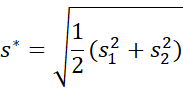
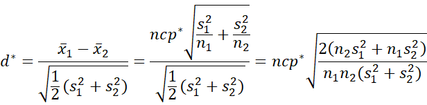
Cohen’s d* is defined by
![]()
where
Hedges’ g* is a less biased version of d*, and is defined by
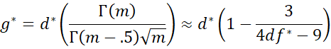
where m = df*/2 and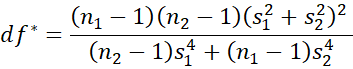
Confidence Interval
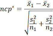
We estimate confidence intervals for d* and g* using the same approach as for d and g (see CI Functions for Effect Sizes d and g). In particular, first we estimate the noncentrality parameter (ncp*) by
Next, we find the confidence interval for ncp* by using the Real Statistics NT_NCP function. The end points of this CI are =NT_NCP(α/2, df*, ncp*) and =NT_NCP(1-α/2, df*, ncp*).
We then use this confidence interval to find a CI for d*. This is done by noting that
Thus, once we have a CI for ncp* we can multiply the end points of this CI by the factor on the right side of the above expression to obtain a CI for d*. Finally, we multiply the end points of the d* CI by the usual factor (involving the gamma function) to obtain a CI for g*.
Example
Example 1: Find the 95% confidence interval of the effect size for Example 2 of Two-Sample t-Test with Unequal Variances.
We show the results of the t-test on the left side of Figure 1 to obtain the needed descriptive statistics. The results on the right side of the figure shows how to estimate the desired confidence intervals.
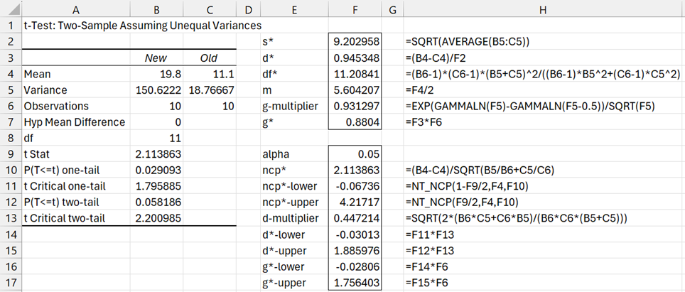
Figure 1 – 95% confidence interval for d* and g* effect sizes
Worksheet Functions
Real Statistics Functions: The Real Statistics Resource Pack provides the following array functions.
T_EFFECT3(m1, m2, s1, s2, n1, n2, lab, alpha, iter) = column array with the values Cohen’s d*, Hedges’ g*, and the lower and upper confidence interval limits for d* and g* based on a two independent sample t-test with unequal variances for sample 1 with mean m1, standard deviation s1 and sample size n1, and sample 2 with mean m2, standard deviation s2 and sample size n2.
TT_EFFECT3(R1, R2, lab, alpha, iter, iter0, prec) = T_EFFECT3(m1, m2, s1, s2, n1, n2, lab, alpha, iter, iter0, prec) where m1 = AVERAGE(R1), s1 = STEV.S(R1), n1 = COUNT(R1), m2 = AVERAGE(R2), s2 = STEV.S(R2) and n2 = COUNT(R2).
alpha is the significance level (default .05). If lab = TRUE (default FALSE) then an extra column of labels is appended to the output.
The last three arguments are as for the NT_NCP function (see Noncentral t Distribution), except that if iter = 0 then the Hedges and Olkin estimate of the confidence interval is employed (iter0 and prec are not used), while if iter > 0 (default 1000) then the estimate of the confidence interval described above based on the noncentrality parameter is used. In this case, iter, iter0, and prec are as for the NT_NCP function (see Noncentral t Distribution).
Example
Referring to the data on the left side of Figure 1, we see that the array formula
=T_EFFECT3(B4,C4,SQRT(B5),SQRT(C5),B6,C6,TRUE)
produces the output shown in Figure 2, which agrees with the results shown on the right side of Figure 1.
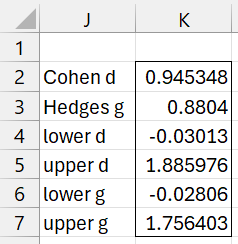
Figure 2 – T_EFFECT3 output
Examples Workbook
Click here to download the Excel workbook with the examples described on this webpage.
References
Delacre, M., Lakens, D., Ley, C., Liu, L., Leys, C. (2021) Why Hedges’ g*s based on the non-pooled standard deviation should be reported with Welch’s t-test
https://psyarxiv.com/tu6mp/download
Howell (2010) Confidence intervals on effect size
https://www.uvm.edu/~statdhtx/methods8/Supplements/MISC/Confidence%20Intervals%20on%20Effect%20Size.pdf
Lecoutre B., (2007) Another look at the confidence intervals for the noncentral t distribution
https://digitalcommons.wayne.edu/jmasm/vol6/iss1/11/
Steiger, J. H., Fouladi, R. T. (1997) Noncentrality interval estimation and the evaluation of statistical models
https://statpower.net/Steiger%20Biblio/Steiger&Fouladi97.PDF
Hedges, L. V. and Olkin, I. (1985) Statistical methods for meta-analysis. Academic Press
https://www.researchgate.net/publication/216811655_Statistical_Methods_in_Meta-Analysis
For some reason, the function I pasted in the previous comment did not come out right. Hoping it comes out correctly here.
g.star.ci <- function(x.bar.1, x.bar.2, s.1, s.2, n.1, n.2, alpha) {
df.star <- (n.1-1)*(n.2-1)*(s.1^2+s.2^2)^2/((n.2-1)*s.1^4 + (n.1-1)*s.2^4)
ncp.star <- (x.bar.1 – x.bar.2)/sqrt(s.1^2/n.1 + s.2^2/n.2)
ncp.star.low <- qt(alpha/2, df.star, ncp.star)
ncp.star.up <- qt(1-alpha/2, df.star, ncp.star)
d.star <- (x.bar.1 – x.bar.2)/sqrt((s.1^2+s.2^2)/2)
m = 170){
J <- (1-3/(4*df.star-9)) # bias correction using approximation
}
if(m < 170){
J <- gamma(m)/(gamma(m-0.5)*sqrt(m)) # bias correction using Gamma function
}
g.star <- d.star*J
g.star.low <- ncp.star.low*sqrt(2*(n.2*s.1^2 + n.1*s.2^2)/(n.1*n.2*(s.1^2+s.2^2)))*J
g.star.up <- ncp.star.up*sqrt(2*(n.2*s.1^2 + n.1*s.2^2)/(n.1*n.2*(s.1^2+s.2^2)))*J
df.g.star.ci <- data.frame(g.star, g.star.low, g.star.up, ncp.star, ncp.star.low, ncp.star.up, d.star, df.star, J, m)
return(df.g.star.ci)
}
This is very helpful. Thank you!
I tried to implement it in R, but I do not get the same values as I see in your example. When the sample sizes are larger, my function delivers closer values to the function that Delacre, et al. (2021) have on their ShinyApp, but it’s still off. From your example, it looks it’s due to what I am using for the Noncentral t Distribution: qt(). Any thoughts?
g.star.ci <- function(x.bar.1, x.bar.2, s.1, s.2, n.1, n.2, alpha) {
df.star <- (n.1-1)*(n.2-1)*(s.1^2+s.2^2)^2/((n.2-1)*s.1^4 + (n.1-1)*s.2^4)
ncp.star <- (x.bar.1 – x.bar.2)/sqrt(s.1^2/n.1 + s.2^2/n.2)
ncp.star.low <- qt(alpha/2, df.star, ncp.star)
ncp.star.up <- qt(1-alpha/2, df.star, ncp.star)
d.star <- (x.bar.1 – x.bar.2)/sqrt((s.1^2+s.2^2)/2)
m = 170){
J <- (1-3/(4*df.star-9)) # bias correction using approximation
}
if(m < 170){
J <- gamma(m)/(gamma(m-0.5)*sqrt(m)) # bias correction using Gamma function
}
g.star <- d.star*J
g.star.low <- ncp.star.low*sqrt(2*(n.2*s.1^2 + n.1*s.2^2)/(n.1*n.2*(s.1^2+s.2^2)))*J
g.star.up <- ncp.star.up*sqrt(2*(n.2*s.1^2 + n.1*s.2^2)/(n.1*n.2*(s.1^2+s.2^2)))*J
#curve(dt(x, df=10000), from=-10, to=10, col = 2)
curve(dt(x, df=df.star, ncp.star), from=-5, to=8, col = 3, add = F)
curve(dt(x, df=df.star), from=-5, to=8, col = 4, add = TRUE)
df.g.star.ci <- data.frame(g.star, g.star.low, g.star.up, ncp.star, ncp.star.low, ncp.star.up, d.star, df.star, J, m)
return(df.g.star.ci)
}
g.star.ci(19.8, 11.1, sqrt(150.6222), sqrt(18.76667), 10, 10, 0.05)
g.star
0.8803999
g.star.low
0.06509529
g.star.up
2.081158
ncp.star
2.113863
ncp.star.low
0.1562955
ncp.star.up
4.996914
d.star
0.9453482
df.star
11.20841
J
0.9312969
m
5.604207
Hello Chritian.
Which values in Figure 1 are different? Both d* and g* values and CI endpoints?
Charles
I get the same d* and g*. The CI endpoints are different for mine. I am using qt() in R for the Noncentral t Distribution.
ncp.star.low and ncp.star.up (and consequently g.star.low and g.star.up) is where we differ.
I looked at the function that Delacre, et al. (2021) wrote and it does not have qt() in it for the Noncentral t Distribution. I think they wrote their own function to calculate it. I reached out to Delacre this morning and hope to hear back.
This is what my function outputs:
g.star
0.8803999
g.star.low
0.06509529
g.star.up
2.081158
ncp.star
2.113863
ncp.star.low
0.1562955
ncp.star.up
4.996914
d.star
0.9453482
df.star
11.20841
J (bias correction using gamma function – your g multiplier)
0.9312969
m
5.604207
using q() from R and nct.ppf() from Python, I got the same for the Noncentral t
Below is the code for Python:
from scipy.stats import nct
nct.ppf(0.025, df=11.20841, nc=2.113863)
0.1562955
Looks like we get the same values for the noncentral t distirbution, although I don’t know what the value of 0.1562955 represents.
Charles
Christian,
I wonder what approach Delacre is using. Have you heard back from him?
Charles
Marie Delacre responded that she was out of office for the month and to reach out to the others on the paper.
I get 0.1562955 for ncp*-lower.
It looks like your NT_NCP function returns -0.03013.
From what it appears to me, it comes down to the way we are calculating the Noncentral t Distribution. I have used functions in R, Python, and SAS to get 0.1562955 for the 2.5 percentile for the Noncentral t with an NCP = 2.113863 and DF = 11.20841.
I figured it out after reading Lecoutre B., (2007) Another look at the confidence intervals for the noncentral t distribution. I changed qt() to conf.limits.nct() from MBESS and now I get the same bounds as you and Marie. Thank you for your website and references!
Christian,
Thanks for the update.
Does this mean that the confidence interval reported on my site is correct?
Charles