Basic Concepts
There is a problem with the analysis given for Example 1 of ANOVA with Repeated Measures for One Within Subjects Factor, namely that the sphericity requirement for repeated-measures ANOVA has not been met. In fact, the requirements for repeated-measures ANOVA are as follows:
- Subjects are independent and randomly selected from the population
- Normality (or at least symmetry) – although overly restrictive it is sufficient for this condition to be met for each treatment (i.e. each column in the analyses that we present)
- Sphericity
Sphericity is an assumption that is stronger than homogeneity of variances and is defined as follows.
Definition 1: Suppose you have k samples of equal size. The data has the sphericity property when the pairwise differences in variance between the samples are all equal.
Such data has the compound symmetry property when all the variances are equal and all the covariances are equal.
Observation: Obviously if there are only two treatments then sphericity is automatically satisfied.
Property 1: Compound symmetry implies sphericity
Proof: Suppose that the data satisfies the compound symmetry property. We consider the case with k = 3; the general case follows similarly. Then the covariance matrix has the form
This can then be simplified to
where ρ is the correlation coefficient. By Property 5 of Basic Concepts of Correlation
From which it follows that the data satisfies the sphericity property.
Observation: The converse is not true since it is easy to give a counter-example.
Sphericity Example
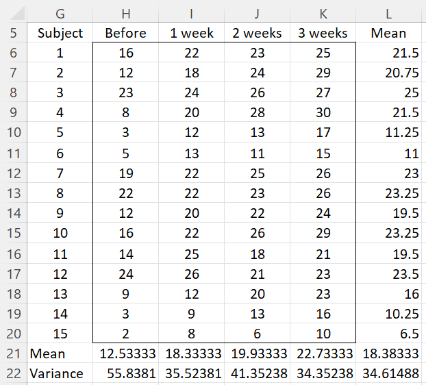
Example 1: Determine whether the data for Example 1 of ANOVA with Repeated Measures for One Within Subjects Factor (repeated in Figure 0) meets the sphericity assumption.
Figure 0 – Data for Example 1
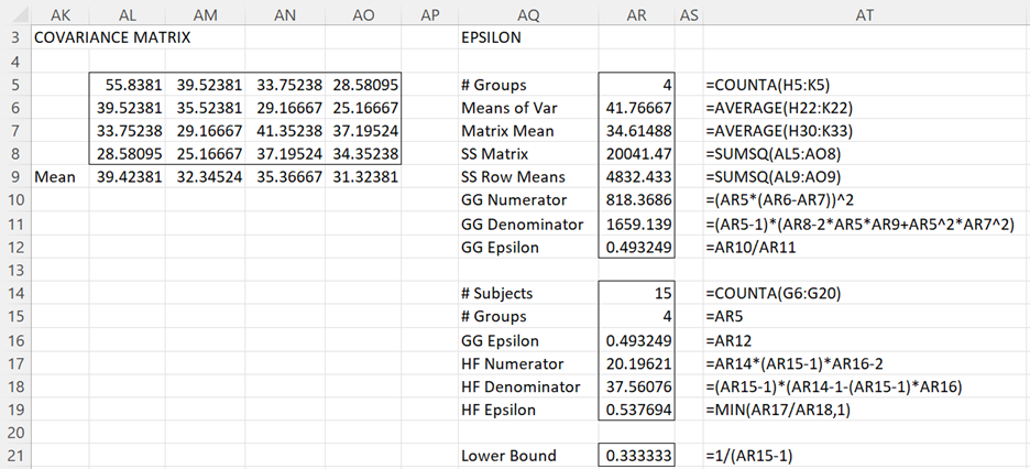
Since we have 4 treatments T0, T1, T2 and T3 the covariance matrix S is an array of form [cij] where cij = cov(Ti, Tj); where i = j, cij = var(Ti). For this example, S is displayed in Figure 1.
Figure 1 – Covariance matrix for Example 1
The worksheet in Figure 1 can be created by highlighting the range W25:Z28 and entering the Real Statistics array formula =COV(H6:K20) described in Method of Least Squares for Multiple Regression. Alternatively, you can use the standard Excel techniques described after Figure 2 of Method of Least Squares for Multiple Regression).
Clearly, the variances (the values along the main diagonal) are different and the covariances are different, and so compound symmetry doesn’t strictly hold, but it is not clear whether these differences are significant.
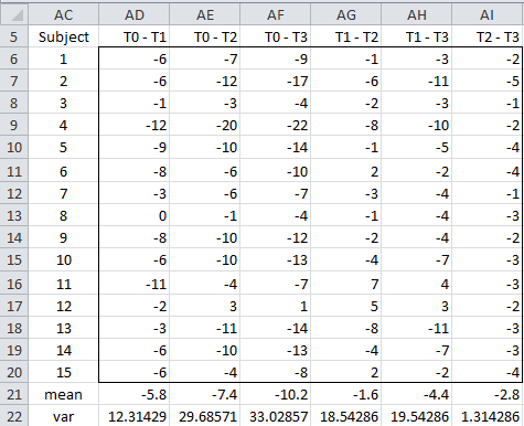
Next, we calculate the variances of the pairwise differences between the treatment values. This can either be calculated directly using the data in Figure 0 or by using Property 5 of Basic Concepts of Correlation
The results for Example 1 are given in Figure 2. For example, cell AD6 is simply the difference between the score for subject 1 before the training and 1 week after (i.e. =H6-I6, referencing the cells in Figure 0) and cell AD22 can be calculated either as =VAR(AD6:AD20) or as =W25+X26-2*X25 (referencing the cells in Figure 1).
Figure 2 – Sphericity for Example 1
Sphericity Correction Factors
From Figure 2, we conclude that the variances of the 6 pairs are clearly not equal, and so it appears that the sphericity assumption has not been met. The resolution is to use a correction factor called epsilon to reduce the degrees of freedom in the F test described in ANOVA with Repeated Measures for One Within Subjects Factor. The most common version of epsilon, due to Greenhouse and Geisser, takes a value between and 1 where k = the number of treatments (i.e. the number of columns, 4 in our example). The value epsilon is given by the formula:
Here S = the sample covariance matrix, = the mean of all the elements in S,
= the mean of all the elements on the diagonal of (i.e. the mean of the variances). For our example, we have
= 0.493 as calculated in cell AR12 of Figure 3 (with references to cells in the worksheet shown in Figure 0).
Figure 3 – GG and HF epsilon for Example 1
In general, is viewed as too conservative (i.e. the correction factor should be higher), and so another common correction factor called the Huynh and Feldt epsilon is also commonly used. It turns out that this factor tends to be slightly too high.
The Huynh and Feldt epsilon is calculated as follows where n = the number of subjects.
For our example, = 0.538, as calculated in cell AR19 of the worksheet in Figure 3.
There is one more commonly used correction factor, namely . This is a lower bound. The correction for sphericity can’t be lower than this.
Worksheet Functions
Real Statistics Functions: The Real Statistics Resource Pack provides the following functions that calculate the GG epsilon and HF epsilon correction factors for both one factor and two-factor repeated-measures ANOVA.
GGEpsilon(R1, ngroups, raw) = Greenhouse and Geisser epsilon value for the data in range R1 where ngroups = the number of independent groups (default 1); if raw = TRUE (default) then R1 contains raw data, otherwise it contains a covariance matrix
HFEpsilon(R1, ngroups, nsubj) = Huynh and Feldt epsilon value for the data in range R1 where ngroups = the number of independent groups (default 1); if nsubj = 0 (default) then R1 contains raw data, otherwise it contains a covariance matrix which is derived from raw data with nsubj subjects (corresponding to rows).
For the one factor case described on this webpage, ngroups = 1. For Example 1, referring to Figure 0, we see that GGEpsilon(H6:K20) = .493 and HFEpsilon(H6:K20) = .538. Referring to Figure 1, we see that GGEpsilon(W25:Z28,1,FALSE) = .493 and HFEpsilon(W25:Z28,1,15) = .538.
Using Sphericity Correction Factors
Example 2: Revise the analysis for Example 1 by using the GG and HF epsilon correction factors.
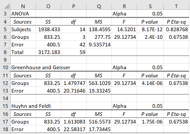
We correct the column and error degrees of freedom by multiplying the dfGroups and dfE values shown in Figure 2 of ANOVA with Repeated Measures for One Within Subjects Factor (and duplicated in the range N3:T8 of Figure 4 below) by an epsilon correction factor. E.g. the revised value of dfE using the Greenhouse and Geisser epsilon is, therefore, dfE ∙ = 42 ∙ .493 = 20.7. These revised values of the degrees of freedom are then used to calculate new values of MSGroups and MSE, and subsequently F = MSGroups/MSE. Note that the revised degrees of freedom won’t necessarily be a whole number. The results are summarized in Figure 4.
Figure 4 – ANOVA analysis using GG and HF epsilon
Examples Workbook
Click here to download the Excel workbook with the examples described on this webpage
Reference
Howell, D. C. (2010) Statistical methods for psychology (7th ed.). Wadsworth, Cengage Learning.
https://labs.la.utexas.edu/gilden/files/2016/05/Statistics-Text.pdf


Dear Charles,
I’ve searched basically all of the internet for an answer, found your page and thought I’d give it a try:
I’m doing quite an extensive research design, with one of the analyses being a 3x4x2 rmANOVA. If Mauchly’s test indicates a violation of the sphericity assumption for one of the main effects and some, but not all of the interaction effects – do I use the epsilon correction only for those effects with violations? And additionally: if some show .75 do I apply Greenhouse-Geisser to some and Huynh-Feldt to others or is consistency thoughout one rmANOVA key?
Thanks in advance!
Best,
Theresa
Hello Theresa,
You should always use a sphericity correction. If one is not really necessary, the correction value will be near 1 anyway, and so will have little impact on the results.
The guidelines are given at https://real-statistics.com/anova-repeated-measures/repeated-measures-anova-tool/
The software tool will output both GG and HF. I don’t think you need to be consistent with which one you report as long as you don’t choose the correction that produces the result you prefer. In practice, what you do here will also depend on your audience (including the publication). They may prefer consistency.
Charles
Dear Professor Zaiontz,
I’d like to thank you for this wonderful site since you explain many vague topics in very straightforward language. My question now:
Is testing sphericity violation enough, and does not necessitate testing whether covariances are significant? And I noticed that the covariance matrix is part of calculating Mauchly’s test, does this mean that the test takes into account the nature of the covariances?
best luck.
Hello Hany,
Thank you for your kind remarks.
For certain tests, sphericity is a requirement (e.g. Repeated Measures ANOVA). For others (e.g. MANOVA) equal covariance matrices is a requirement. Sphericity does not imply equal covariances though.
Charles
Thank you, Sir.
Hi Charles,
“Sphericity is an assumption that is stronger than homogeneity of variances”.
What does “stronger” mean here?
In this case, it means that if the sphericity assumption holds, then so does the homogeneity of variances assumption.
Charles
Crystal clear answer.
Thanks.
Charles,
Can you check the function set up of HFEpsilon when it uses a covariance matrix data as the range value? When I conducted the function using Ex 1, the HFEpsilon function using the original input data as the data range, the function gave the same value as the manually calculated value (ie, 0.538), which is the same as you stated in the text. But, when I used the covariance matrix range as the range data (ie, HFEpsilon (covariance matrix range, 1)), then the function gave a different value (0.420). I repeated the same function without the ngroups argument as you did in the text. And the same 0.420 showed.
-Sun
Charles,
Please disregard the previous comments. I should have entered a value for nsubj when I executed the function.
But, I have one other question which led me a confusion at the first place. When the input range value is the original data, shouldn’t we enter the second and third arguments of the HFEpsilon function. Instead of HFEpsilon(original data range) as shown in the text, the second and third arguments should be 1 and 0 like HFEpsilon(original data range, 1, 0).
Hello Sun,
The default for the second argument is 1 and the default for the third argument is 0. This is why both arguments can be omitted. I will shortly make this clearer on the webpage.
Charles
Sun,
I think that you have already figured out that the third argument must be set to 15.
Charles
Dead Charls
I would ask a quastion : “epsilon correction must be applied only on the F test of ANOVA(repeated measures), or there are corrections to the multiple comparison after ANOVA too? I don’t ask for the specific correction in Bonferroni, Tukey, etc but if theese correctionss (Bonferroni, Tukey,etc) must be corrected for Sphericity. ”
Thanks
Dear Charles,
For clarification, when applying the 0.75 rule of thumb for determining whether to use the GG or HF epsilon, what value are we comparing to 0.75?
For my data, I have a GG epsilon of 0.444 and a HF epsilon of 1.00.
Regards,
Tom
Tom,
I would compare the .75 with the GG epsilon value. With such a low value, it does seem that sphericity is being violated. You might consider using MANOVA.
Charles
Dear Charles,
Thank you for your informative and very practical web site. My question relates to sphericity tests applied to two way ANOVAs. For the single factors it is clear the same calculations would apply as for the one way case, but what about calculating sphericity for the interaction term? Is the correct covariance matrix one that consists of all values of both factors?
Regards,
James
James,
I think you are referring to the case described on the following webpage:
https://real-statistics.com/anova-repeated-measures/one-between-subjects-factor-and-one-within-subjects-factor/
Charles
Dear Charles!
I have a question with regards to the “One repeated measures procedure”.
Assume, I would like to compare overnights of 100 different hotels between the years 1999, 2000, and 2001. The typical way to check whether sphericity can be assumed – at least to my knowledge – is first to run Mauchly’s test of sphericity or John, Nagao and Sugiura’s test of sphericity. If this test is significant, we have a look at the Greenhouse-Geisser epsilon to decide upon whether to apply the Greenhouse-Geisser or Huyhn-Feldt correction (the .75 rule).
My question is, how to quickly check with the Realstat add-ins whether the sphericity assumption in such a case is violated, as the “One repeated measures procedure” implemented in the Realstat add-ins does not give me information about sphericity, or does it?
Many thanks in advance for your response!
Best wishes,
Christian
Christian,
The Real Statistics add-in does provide information about sphericity. See, for example, Figure 6 on the referenced webpage.
Also, you don’t really need to test for sphericity using Mauchly’s test or John, Nagao, Sugiura’s test. You can simply apply the GG or HF correction.
Charles
Dear Dr. Charles,
first of all thank you very much for all the help you provide us through your website and statistical tools for excel!
I would like to have your comments about this question.
I have a one-factor repeated measures ANOVA, related to clinical data from a group of subjects that have been measured before receiving a treatment and then measured again after the treatment, for 7 times during a given time period.
The 8 groups of data show a relevant deviation from sphericity (GGepsilon = 0.54, HFepsilon = 0.59).
Anyway, after applying the GG or HF correction, the ANOVA resulted significant (p = 0.022) so I wish to proceed with post-hoc comparisons.
I am not interested to all pairwise comparison, but only in comparing pre-treatment group with each post-treatment group, so a total of 7 not-orthogonal contrasts.
Given that the sphericity assumption is largely violated, can I still perform paired t-test between groups of interest with the Bonferroni correction (t-test alpha = 0.05/7), or this is not recommended?
I tried to search on the web, but it seems that there is not good agreement about this issue, so I would appreciate to have your opinion about.
Thank you very much
Piero
Piero,
Since there is no sphericity issue for pairwise tests, I can’t think of any reason why you couldn’t do exactly what you propose (or use the Dunn/Sidak correction).
Charles
Dear Charles
Thank you very much for your help and time, it’s very appreciated as well as the precious work you do with this website and statistic tools of yours! I wouldn’t know what to do without it!
I didn’t make myself clear very much with my question about the test but I think I figured it out – next thing I have to do with my data is do a Tukey’s HSD test. However, I am not quite sure, therefore you may can help me with this:
I have a study where the teeth of 40 subjects were measured over time 5 times (repeated measures in the same subjects) and the L (ligthness), b (yellow – blue colour), a (green – red colour), C (colour intensity) and h (hue) values are recorded. From the start of the study/analysis I know that there will be no change in the h and a values – so these parameters are not interesting for me, only the L, b and C value I would like to analyse closer. Now I thought I would do the analysis the following way: perform with every parameter (L, b, C) seperately an ANOVA repeated measure with one within subject factor analysis followed by a Tukey’s HSD test with Bonferroni correction. Is that a good approach? Thank you very much for your help – statistics is really difficult for non-statisticans!
Claudine,
I agree that statistics can be difficult, not just for non-statisticians, but for everyone. Since you have three dependent variables, it sounds like you might benefit from using MANOVA (the multivariate analog to ANOVA). This will take into account any correlations between the dependent variables. You can read more about this on the webpage MANOVA, especially Two Factor Multivariate Repeated Measures.
Charles
Dear Charles
One more question: and then what test do I need to do, to find out between which groups there is a significant difference?
Thanks a lot for your help!
Claudine
Claudine,
I don’t know how to calculate whether there is a significant difference between the groups; if a significance test is required you should use Mauchly’s test. However, as I said in my previous response, generally it is better to use the GG or HF correction factor. Another rule of thumb here is that if the epsilon-GG < .75 use the GG correction; otherwise use the HF correction. Charles
Dear Charles
Thank you very much for your Analysis Tool and explanations – it’s very helpful!
I used it do to a one within subjects factor analysis where I have subjects that were measured over time 5 times and got an output similar to figure 6. What I don’t understand is how I see out of the output data whether sphericity is meet or not – and therefore which data I have to report, df-corrected (GG; HF) or the not corrected Anova data? Is there a rule or easy way to see it? Do I have to do a “manual” analysis like shown in figure 2 and if so then what “difference” between the pairwise differences in variance between samples is supposed to be fair enough to meet the sphericity property of “equal”?
Dear Claudine,
Generally, it is better to simply use either the GG or HF correction factor and not worry about whether the sphericity assumption is met or not. Of course if the corrected test values are pretty similar to the uncorrected values then probably sphericity wasn’t much of a problem. Regarding which correction factor to use, some people use GG and some use an average between GG and HF. Additional information is given on the referenced webpage.
If you need to calculate the sphericity you can manually perform the calculations shown in Figure 2. Alternatively you can use Mauchly’s test as described in Additional Information about Sphericity.
Charles