Markov Chains Basic Concepts

Introduction

In a Markov chain process, there are a set of states and we progress from one state to another based on a fixed probability. Figure 1 displays a Markov chain with three states. E.g. the probability of transition from state C to state A is .3, from C to B is .2 and from C to C is .5, which sum up to 1 as expected.

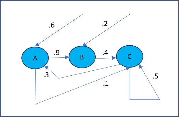
Figure 1 – Markov Chain transition diagram

The important characteristic of a Markov chain is that at any stage the next state is only dependent on the current state and not on the previous states; in this sense it is memoryless.

Definitions

Definition 1: A (finite) Markov chain is a stochastic process x₀, x₁, … such that each x_i belongs to some finite set S such that the probability that x_i+1 has outcome s in S only depends on the value of x_i, i.e.

P(x_i+1 = s | x₀ = s₀, x₁ = s₁, …, x_i = s_i) = P(x_i+1 = s | x_i = s_i)

for any states s₀, s₁, …, s_i, s.

We will further assume that the Markov chains are time-homogeneous (i.e. stationary), i.e. for any i

P(x_i+1 = s | x_i = r) = P(x₁ = s | x₀ = r)

Now define the (one-step) transition probability from state r to s by

p_rs = P(x_i+1 = s | x_i = r)

Thus, clearly for all r, s in S

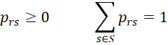
as in Property 1 of Discrete Probability Distributions.

A Markov chain is completely determined by the distribution of the initial state x₀ and the transition probabilities p_rs.

k-step transitions

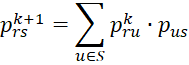
Now define the k-step transition probability from state r to s by

Clearly p¹_rs = p_rs.

Properties

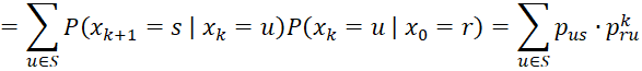
Property 1 (Chapman-Kolmogorov): For any k

Proof: Using the law of conditional probabilities and the Markov chain assumptions, we have

Property 2: Assuming that x₀ = r, the expected number of times x_i = s for 1 ≤ i ≤ n is

Proof: For fixed r and s, define the stochastic process y_i as follows

Thus

Now define the random variable

It now follows that

which proves the result.

Transition Matrix

Definition 2: Assuming that the set of states is specified as S = {1,…, n}, we define the n × n (one-step) transition matrix to be P = [p_ij] (here we are using indices such as i, j to represent the states).

It now follows from Property 1 that P^k = [p^k_ij] where P^k is the matrix P multiplied by itself k times, i.e. P^k is the k-step transition matrix.

A Markov chain can also be described by a transition diagram which consists of the finite states connected by arrows which represent the transition probabilities, such as shown in Figure 1.

Definition 3: A state s is called an absorbing state if p_ss = 1. A Markov chain is an absorbing Markov chain if there are one or more absorbing states such than any state eventually arrives at an absorbing state.

If a Markov chain arrives at an absorbing state then it stays in that state forever. An absorbing Markov chain eventually arrives at an absorbing state no matter what the initial state is.

References

Fewster, R. (2014) Markov chains
https://www.stat.auckland.ac.nz/~fewster/325/notes/ch8.pdf

Pishro-Nik, H. (2014) Discrete-time Markov chains
https://www.probabilitycourse.com/chapter11/11_2_1_introduction.php

Norris, J. (2004) Discrete-time Markov chains
https://www.statslab.cam.ac.uk/~james/Markov/

Lalley, S. (2016) Markov chains
https://galton.uchicago.edu/~lalley/Courses/312/MarkovChains.pdf

Konstantopoulos, T. (2009) Markov chains and random walks
https://www2.math.uu.se/~takis/L/McRw/mcrw.pdf