More Numerical Differential Equation Methods

Objective

Using the approach described in Euler’s Forward Method for solving differential equations, we now explore three other methods. These are Euler’s backward method, the Trapezoid method, and the Runge-Kutta method.

Euler’s Backward Method

This method is based on the following approximation to a derivative.

It follows that

This means that the system is characterized by

y_i+1 = y_i + h f(x_i+1, y_i+1)          y₀ = constant

Since we have y_i+1 on both sides of the equation, we don’t have an explicit solution. Instead, we need to find the root of an equation of form

y_i+1 – y_i – h f(x_i+1, y_i+1) = 0

e.g. by using Newton’s method. Alternatively, we can make an initial estimate for y_i+1 using Euler’s forward method, namely

We then apply a fixed point iterative approach as follows

Fortunately, convergence is usually quite rapid. One iteration is often sufficient, in which case

y_i+1 = y_i + h f(x_i+1, y_i + f(x_i, y_i)) 

Example 1: Repeat Example 2 of Euler’s Forward Method using Euler’s Backward method with two iterations.

The result is shown in Figure 1.

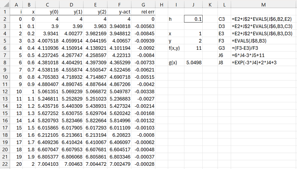
Figure 1 – Euler Backward Method

For this example, the results are fairly similar to those obtained for Example 2 in Euler’s Forward Method.

Trapezoid Method

As we see in Numerical Integration

This estimate is especially accurate over a small interval [a, b]

Thus to solve

y′(x) = f(x, y(x))

we can take the integral of both sides from x_i to x_i+1 to obtain

and so

This motivates the iterative process

As for the Euler Backward algorithm, this requires an implicit solution. A similar approach is to use the Euler Forward algorithm for the initial guess.

and then

Note that the Trapezoid method with one iteration is called Heun’s method.

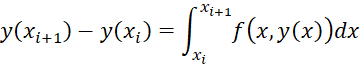
Example 2: Repeat Example 1 using the Trapezoid method with two iterations.

The results are shown in Figure 2.

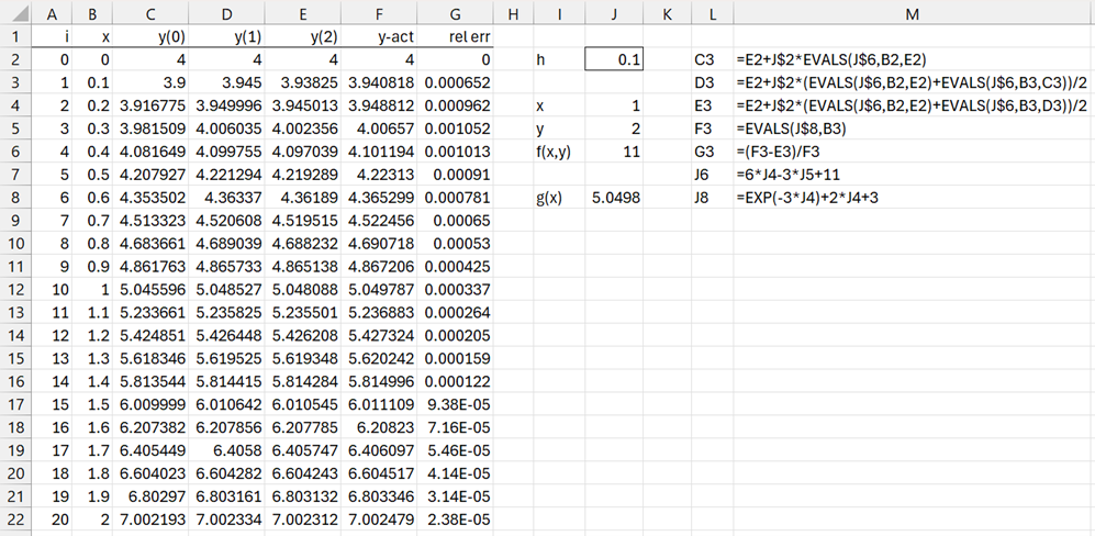
Figure 2 – Trapezoid method

This approach provides better estimates for y(2), with relative error of 0.00238%.

Runge-Kutta (RK2) method

This method attempts to make a better approximation by using an expanded version of the Taylor series. This method uses the following explicit iterative approach:

y_i+1 = y_i + hF(x_i, y_i) 

where

This means that

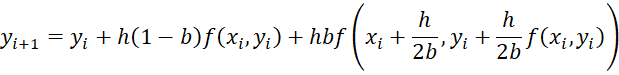
Typical choices for b are 1/2, 2/3, 3/4, and 1. The case where b = 1/2 is Heun’s method. b = 1 results in the midpoint method, and b = 2/3 is Ralston’s  method.

Example 3: Repeat Example 1 using the Runge-Kutta Method with b = ½.

The results are shown in Figure 3.

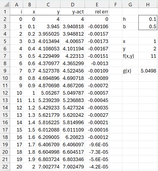
Figure 3 – Runge-Kutta Method

Here, cell C3 contains the formula

=C2+H$2*(1-H$3)*EVALS(H$7,B2,C2)+ H$2*H$3*EVALS(H$7,B2+H$2/(2*H$3),C2+H$2/(2*H$3)*EVALS(H$7,B2,C2))

Not surprisingly, the estimate for y(2) is comparable to the Trapezoid method.

Runge-Kutta (RK4) method

There is an extended version of the Runge-Kutta method described above. This method uses the following iterative approach:

k₁ = hf(x_i, y_i, z_i)

k₂ = hf(x_i+h/2, y_i+k₁/2, z_i+m₁/2)

k₃ = hf(x_i+h/2, y_i+k₂/2, z_i+m₂/2)

k₄ = hf(x_i+h, y_i+k₃, z_i+m₃)

y_i+1 = y_i + (k₁+2k₂+2k₃+k₄)/6

See Differential Equations Analysis Tool for an example using RK4.

Interpolation

Example 4: Repeat Example 3 to find the solution to the differential equation when x = 1.12.

We have two choices. We could select a value of h that evenly divides 1.12. E.g. h = .01 or h = .02. If, however, we stick with h = .1, then we can use interpolation. To keep things simple, we will use linear interpolation (see Interpolation), as described in Figure 4 (with reference to the analysis shown in Figure 3).

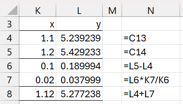
Figure 4 – Linear interpolation

The linear interpolation estimate is y(1.12) = 5.277238 (cell L8).

Examples Workbook

Click here to download the Excel workbook with the examples described on this webpage.

References

Strang, G., Herman, E., Seeburger, P. (2025) Introduction to differential equations
https://math.libretexts.org/Courses/Monroe_Community_College/MTH_211_Calculus_II/Chapter_8%3A_Introduction_to_Differential_Equations/8.1%3A_Basics_of_Differential_Equations

Atkinson, K., Han, W., Stewart, D. (2009) Numerical solutions to ordinary differential equations. Wiley-Interscience
https://homepage.math.uiowa.edu/~atkinson/papers/NAODE_Book.pdf

Wilson, H. J. (2025) Ordinary differential equations
https://www.ucl.ac.uk/~ucahhwi/GM01/ODE_extra.pdf

Wikipedia (2025) Numerical methods for ordinary differential equations
https://en.wikipedia.org/wiki/Numerical_methods_for_ordinary_differential_equations