For a known continuous distribution, we can estimate facts about the order statistics (as well as the median or mean) for a sample from this distribution by using Monte Carlo simulation.
Examples
Example 1: Estimate the median for a sample of size 10 from a population with a gamma distribution with parameters alpha = 100 and beta = .13. Also, find the standard error of this estimate and a 95% confidence interval of this estimate.
We create 200 simulated samples from this distribution, as shown in range E2:N201 of Figure 1 (only the first 10 samples are shown). We generate each element in this range via the worksheet formula =GAMMA.INV(RAND(),100,0.13).
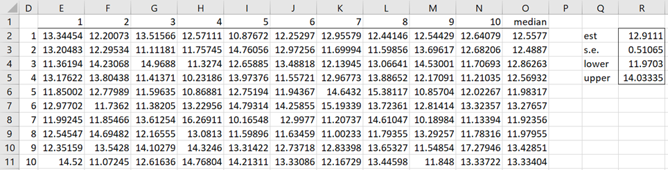 Figure 1 – Monte Carlo simulation
From this point on, the approach is similar to that used for bootstrapping. The result is shown in range Q2:R5. For example, the estimated median of 12.9111 is shown in cell R2 using the formula =AVERAGE(O2:O201). Note that this estimate is pretty close to the population median of 12.9567, as calculated by the formula =GAMMA.INV(.5,100,.13). Increasing the number of simulations will tend to improve the accuracy of the results.
Worksheet Functions
Real Statistics Functions: The Real Statistics Resource Pack provides the following two array functions. These functions refer to a distribution dist (“uniform”, “normal”, etc.) with the specified parameters as described for the MEAN_DIST and VAR_DIST functions (see Distribution Property Functions).
ORDER_SIM(k, n, lab, iter, alpha, dist, param1, param2, param3): returns a column array with the estimated value of the kth order statistic based on iter (default 1000) simulated samples of size n from the distribution specified by dist with the specified parameters; the output also contains the standard error of the estimate along with the 1–alpha confidence interval (default for alpha is .05).
If k = 0 (default) then the output estimates the median instead of the kth order statistic. If lab = TRUE (default FALSE), then a column of labels is appended to the output.
Note that the formula =ORDER_SIM(0,10,TRUE,,,”gamma”,100,0.13) produces output similar to that shown in range Q2:R5 in Figure 1.
RANGE_SIM(j, k, n, lab, iter, alpha, dist, param1, param2, param3): returns a column array with the estimated value of the x(k) – x(j) range statistic based on iter (default 1000) simulated samples of size n from the distribution specified by dist with the specified parameters; the output also contains the standard error of the estimate along with the 1–alpha confidence interval (default for alpha is .05).
E.g. the expected value for the x(10) – x(1) range statistic (along with the standard error of the estimate and 95% confidence interval) for a sample of size 10 from the Gamma distribution with parameters alpha = 100 and beta = .13 can be calculated using the following array formula: =RANGE_SIM(1,10, ,10,TRUE,,,”gamma”,100,0.13). The results are shown in Figure 2.
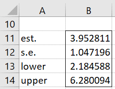
Figure 2 – Simulation of the range statistic
Examples Workbook
Click here to download the Excel workbook with the examples described on this webpage.
References
Chen, P-N (2008) Basic theories on order statistics
Reference is no longer available
Omondi, O. C. (2016) Order statistics of uniform, logistic and exponential distributions
http://erepository.uonbi.ac.ke/bitstream/handle/11295/97307/MSc_Project2016.pdf?sequence=1&isAllowed=y
Ma D. (2010) The distribution of the order statistics. A Blog on probability and statistics
https://probabilityandstats.wordpress.com/2010/02/20/the-distributions-of-the-order-statistics/
Border, K. C. (2016) Lecture 15: Order statistics; conditional expectation. Caltech
https://healy.econ.ohio-state.edu/kcb/Ma103/Notes/Lecture15.pdf