Normal Confidence Intervals for Percentiles

Objective

In Confidence Intervals for Order Statistics, Medians and Percentiles, and Confidence Intervals for Quartiles and Percentiles we show how to estimate confidence intervals for order statistics, the median, quartiles, and percentiles using a binomial distribution approach. We now show how to modify this approach by using the fact that the normal distribution can be used to approximate the binomial distribution (see Relationship Normal and Binomial Distributions).

Basic Concepts

If the sample is large enough (say n ≥ 20), we can also use the normal approximation to the binomial distribution. For any value u, let v = the number of elements in the sample < u. As we saw in the proof of Property 1 of Confidence Intervals for Order Statistics, Medians and Percentiles, v ∼ B(n, p). Using the normal approximation, we have v ∼ N(μ, σ²) where

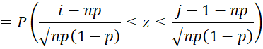
Thus, z ∼ N(0,1)  where z = (v–μ)/σ, and so

After applying a .5 continuity factor, we get

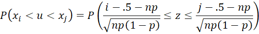
This probability can be calculated in Excel using the NORM.S.DIST function or more directly using the following formula:

=NORM.DIST(j-.5,np,SQRT(np(1-p)),TRUE)-NORM.DIST(i-.5,np,SQRT(np(1-p)),TRUE)

Note that the normal approximation can be used to estimate the confidence interval for order statistics, the median or quartiles as well, although usually the binomial estimate is sufficient. For quartiles and percentiles, the normal approximation enables us to obtain a symmetric confidence interval as described below.

Example using Normal Estimation

Example 1: Estimate the 60% percentile and its 95% confidence interval based on the sample from Example 1 of Confidence Intervals for Order Statistics, Medians and Percentiles (the data is repeated on the left side of Figure 1).

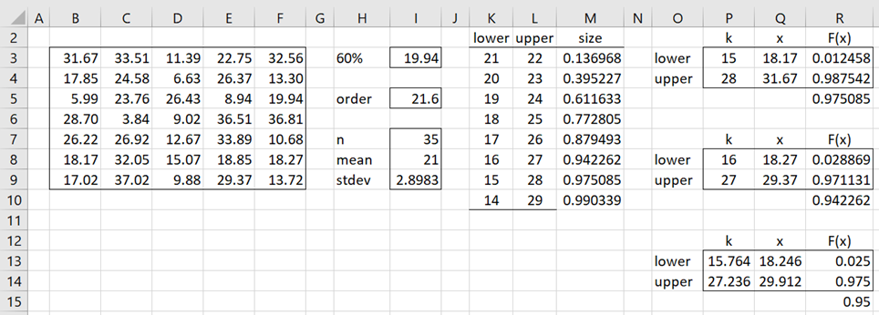
Figure 1 – Confidence interval for 60% percentile

The 60% percentile of the sample in Figure 1 is 25.564 as calculated by the formula =PERCENTILE.EXC(B3:F9,.6). This value is between the 24.58 and 26.22 sample values. Alternatively, this value can be calculated as follows.

This time, instead of using the binomial estimate for each interval, we use a normal approximation with mean np = 35(.6) = 21 (cell I8) and variance = np(1-p) = 21(1-.6) = 8.4, and the standard deviation is the square root of 8.4 as shown in cell I9. E.g. the formula in cell M3 is

=NORM.DIST(L3-0.5,I$8,I$9,TRUE)-NORM.DIST(K3-0.5,I$8,I$9,TRUE)

We see that the 95% confidence interval is closest to the interval (x₍₁₆₎, x₍₂₇₎) = (18.27, 29.37). This interval is actually a 94.23% confidence interval. Note too that since the “order statistic” of 21.6 is not exactly halfway between 21 and 22, the confidence interval is not completely symmetric.

Use of Goal Seek

We can obtain a symmetric interval if we are willing to use interpolation. This can be done as shown in Figure 2 using Excel’s Goal Seek capability (which is accessible via Data > What-if Analysis|Goal Seek). Here, we set the offset in cell U3 to any initial value. The formulas in cells U6 and U7 are =I5-U3 and =I5+U3, respectively. The formulas in column W are the same as those used in column R (based on the normal approximation).

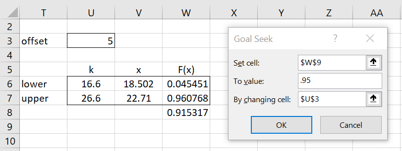
Figure 2 – Goal Seek initialization

After clicking on the OK button, we obtain the result shown in Figure 3.

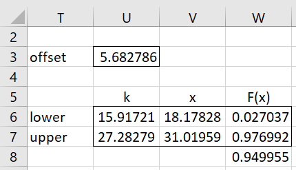
Figure 3 – 95% confidence interval

This results in an offset of 5.682786 (cell U3) and so the 95% confidence interval is (a, b) where a = the weighted average between x₍₁₅₎ and x₍₁₆₎ using the weights .91721 and .09279 respectively. Similarly, b = the weighted average between x₍₂₇₎ and x₍₂₈₎ using the weights .28279 and .71721 respectively. Using these same weights, we obtain the confidence interval (18.17828, 31.01959).

Here, for example, the formula in cell V6 is

=SMALL(B3:F9,INT(U6))*(U6-INT(U6))+SMALL(B3:F9,INT(U6)+1)*(1-U6+INT(U6))

The formula in cell V7 is similar.

Examples Workbook

Click here to download the Excel workbook with the examples described on this webpage.

References

Penn State University (2021) Distribution free confidence intervals for percentiles
https://online.stat.psu.edu/stat415/lesson/19