Basic Concepts for ANOVA

Introduction

We start  our description of ANOVA with the one-factor case. We will define the concept of factor elsewhere, but for now, we simply view this type of analysis as an extension of the t-tests that are described in Two Sample t-Test with Equal Variances and Two Sample t-Test with Unequal Variances. We begin with an example which is an extension of Example 1 of Two Sample t-Test with Equal Variances.

Example

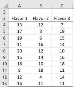
Example 1: A marketing research firm tests the effectiveness of three new flavorings for a leading beverage using a sample of 30 people, divided randomly into three groups of 10 people each. Group 1 tastes flavor 1, group 2 tastes flavor 2 and group 3 tastes flavor 3.  Each person is then given a questionnaire that evaluates how enjoyable the beverage was. The scores are as in Figure 1. Determine whether there is a perceived significant difference between the three flavorings.

Figure 1 – Data for Example 1

Since the people in the study are assigned to the groups at random, this sort of experiment is said to be a completely random experimental design. We can consider the flavors are the independent variable (with three categorical values) and the scores from the questionnaires as the dependent variable.

Our null hypothesis is that any difference between the three flavors is due to chance.

H₀: μ₁ = μ₂ = μ₃

        H₁: μ₁ ≠ μ₂ or μ₁ ≠ μ₃ or μ₂ ≠ μ₃

We interrupt the analysis of this example to give some background, after which we will resume the analysis.

Basic Definitions

Definition 1: Suppose we have k samples, which we will call groups (or treatments); these are the columns in our analysis (corresponding to the 3 flavors in the above example). We will use the index j for these. Each group consists of a sample of size n_j. The sample elements are the rows in the analysis. We will use the index i for these.

Suppose the jth group sample is

and so the total sample consists of all the elements

We will use the abbreviation x̄_j for the mean of the jth group sample (called the group mean) and x̄ for the mean of the total sample (called the total or grand mean).

Let the sum of squares for the jth group be

We now define the following terms:

SS_T is the sum of squares for the total sample, i.e. the sum of the squared deviations from the grand mean. SS_W is the sum of squares within the groups, i.e. the sum of the squared means across all groups. SS_B is the sum of the squares between-group sample means, i.e. the weighted sum of the squared deviations of the group means from the grand mean.

Where

we also define the following degrees of freedom

Finally, we define the mean square as

and so

Summarizing:

Observations: Clearly MS_T is the variance for the total sample. MS_W is the weighted average of the group sample variances (using the group df as the weights). MS_B is the variance for the “between sample” i.e. the variance of {n₁x̄₁, …, n_kx̄_k}.

Properties

Property 1: If a sample is made as described in Definition 1, with the x_ij independently and normally distributed and with all σ_j² equal, then

Property 1 can be used to calculate confidence intervals for MS_T, MS_B and MS_W.

Property 2:

Click here for a proof of Properties 1 and 2.

Structural Model

Definition 2: Using the terminology from Definition 1, we define the structural model as follows. First, we estimate the group means from the total mean: = μ + a_j where a_j denotes the effect of the jth group (i.e. the departure of the jth group mean from the total mean). We have a similar estimate for the sample of x̄_j = x̄ + a_j.

The null hypothesis is now equivalent to

         H₀: a_j = 0 for all j

Similarly, we can represent each element in the sample as x_ij = μ + α_j + ε_ij where ε_ij denotes the error for the ith element in the jth group. As before we have the sample version x_ij = x̄ + a_j + e_ij where e_ij is the counterpart to ε_ij in the sample.

Also ε_ij = x_ij – (μ + α_j) = x_ij – μ_j and similarly, e_ij = x_ij – x̄_j.

Observation: Since

it follows that

and so
for any j, as well as

If all the groups are equal in size, say n_j = m for all j, then

i.e. the mean of the group means is the total mean. Also

Property 3:

Click here for a proof of Property 3.

Observations

MS_B is a measure of the variability of the group means around the total mean. MS_W is a measure of the variability of each group around its mean, and, by Property 3, can be considered a measure of the total variability due to error. For this reason, we will sometimes replace MS_W, SS_W and df_W by MS_E, SS_E and df_E.

In fact,

If the null hypothesis is true, then α_j = 0, and so

While if the alternative hypothesis is true, then α_j ≠ 0, and so

If the null hypothesis is true then MS_W and MS_B are both measures of the same error and so we should expect F = MS_B / MS_W to be around 1. If the null hypothesis is false we expect that F > 1 since MS_B will estimate the same quantity as MS_W plus group effects.

In conclusion, if the null hypothesis is true, and so the population means μ_j for the k groups are equal, then any variability of the group means around the total mean is due to chance and can also be considered an error.

Thus the null hypothesis becomes equivalent to H₀: σ_B = σ_W (or in the one-tail test, H₀: σ_B ≤ σ_W). We can therefore use the F-test (see Two Sample Hypothesis Testing of Variances)  to determine whether or not to reject the null hypothesis.

Relationship with F distribution

Property 4: If a sample is made as described in Definition 1, with the x_ij independently and normally distributed and with all μ_j equal and all equal, then

Proof: The result follows from Property 1 and Theorem 1 of F Distribution.

Example resumed

Example 1 (continued): We now resume our analysis of Example 1 by calculating F and testing it as in Property 4.

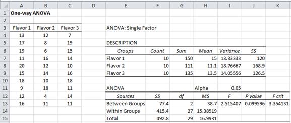
Figure 2 – ANOVA for Example 1

Based on the null hypothesis, the three group means are equal, and as we can see from Figure 2, the group variances are roughly the same. Thus we can apply Property 4. To calculate F we first calculate SS_B and SS_W. Per Definition 1, SS_W is the sum of the group SS_j (located in cells J7:J9). E.g. SS₁ (in cell J7) can be calculated by the formula =DEVSQ(A4:A13). SS_W (in cell F14) can therefore be calculated by the formula =SUM(J7:J9).

The formula =DEVSQ(A4:C13) can be used to calculate SS_T (in cell F15), and then per Property 2, SS_B = SS_T – SS_W = 492.8 – 415.4 = 77.4. By Definition 1, df_T = n – 1 = 30 – 1 = 29, df_B = k – 1 = 3 – 1 = 2 and df_W = n – k = 30 – 3 = 27. Each SS value can be divided by the corresponding df value to obtain the MS values in cells H13:H15. F = MS_B / MS_W = 38.7/15.4 = 2.5.

F test

We now test F as we did in Two Sample Hypothesis Testing of Variances, namely:

p-value = F.DIST.RT(F, df_B, df_W) = F.DIST.RT(2.5, 2, 27) = .099596 > .05 = α

F_crit = F.INV.RT(α, df_B, df_W) = F.INV.RT(.05, 2, 27) = 3.35 > 2.5 = F

Either of these shows that we can’t reject the null hypothesis that all the means are equal.

As explained above, the null hypothesis can be expressed by H₀: σ_B ≤ σ_W, and so the appropriate F test is a one-tail test, which is exactly what F.DIST.RT and F.INV.RT provide.

We can also calculate SS_B as the square of the deviations of the group means where each group mean is weighted by its size. Since all the groups have the same size this can be expressed as =DEVSQ(H7:H9)*F7.

SS_B can also be calculated as DEVSQ(G7:G9)/F7. This works as long as all the group means have the same size.

Data Analysis Tool

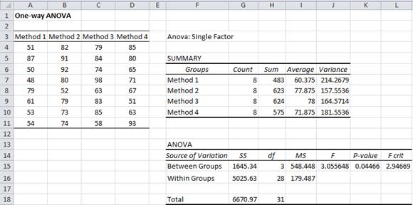
Excel Data Analysis Tool: Excel’s Anova: Single Factor data analysis tool can also be used to perform analysis of variance. We show the output for this tool in Example 2 below.

The Real Statistics Resource Pack also contains a similar data analysis tool that also provides additional information. We show how to use this tool in Example 1 of Confidence Interval for ANOVA.

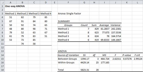
Example 2: A school district uses four different methods of teaching their students how to read and wants to find out if there is any significant difference between the reading scores achieved using the four methods. It creates a sample of 8 students for each of the four methods. The reading scores achieved by the participants in each group are as follows:

Figure 3 – Anova: Single Factor data analysis tool

This time the p-value = .04466 < .05 = α, and so we reject the null hypothesis, and conclude that there are significant differences between the methods (i.e. all four methods don’t have the same mean).

Note that although the variances are not the same, as we will see shortly, they are close enough to use ANOVA.

Observation: We next review some of the concepts described in Definition 2 using Example 2.

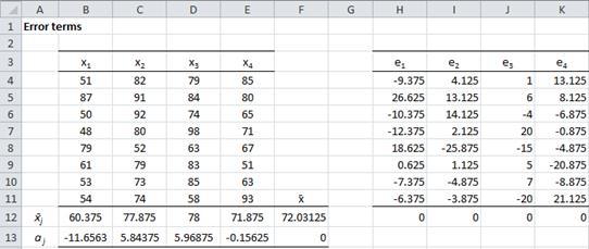
Figure 4 – Error terms for Example 2

From Figure 4, we see that

• x̄ = total mean = AVERAGE(B4:E11) = 72.03 (cell F12)
• mean of the group means = AVERAGE(B12:E12) = 72.03 = total mean
• = 0 (cell F13)
•  = 0 for all j (cells H12 through K12)

We also observe that Var(e) = VAR(H4:K11) = 162.12, and so by Property 3,

and so

which agrees with the value given in Figure 3.

Example with unequal groups sizes

In Examples 1 and 2, all the group sizes were equal. This doesn’t have to be the case, as we see from the following example.

Example 3: Repeat the analysis for Example 2 where the last participant in group 1 and the last two participants in group 4 leave the study before their reading tests were recorded.

Figure 5 – Data and analysis for Example 3

Using Excel’s data analysis tool we see that p-value = .07276 > .05 = α, and so we cannot reject the null hypothesis and conclude there is no significant difference between the means of the four methods.

Generalizing t-test for two samples

MS_W can also be calculated as a generalized version of Property 1 of Two Sample t-Test with Equal Variances. There we had

When there are more than two groups, MS_W can be calculated as a generalized version of the above formula

From Figure 6, we see that we obtain a value for MS_W in Example 3 of 177.1655, which is the same value that we obtained in Figure 5.

Figure 6 – Alternative calculation of MS_W

Calculating SS between groups

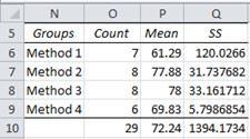
As we did in Example 1 we can calculate SS_B as SS_B = SS_T – SS_W. We now show alternative ways of calculating SS_B for Example 3.

Figure 7 – Alternative calculation of SS_B

We first find the total mean (the value in cell P10 of Figure 7), which can be calculated either as =AVERAGE(A4:D11) from Figure 5 or =SUMPRODUCT(O6:O9,P6:P9)/O10 from Figure 7. We then calculate the square of the deviation of each group mean from the total mean. E.g. for group 1, this value (located in cell Q6) is given by =(P6-P10)^2. Finally, SS_B can now be calculated as =SUMPRODUCT(O6:O9,Q6:Q9).

Worksheet Functions

Real Statistics Functions: The Real Statistics Resource Pack contains the following supplemental functions for the data in range R1:

SSW(R1, b) = SSW	dfW(R1, b) = dfW	MSW(R1, b) = MSW
SSBet(R1, b) = SSB	dfBet(R1, b) = dfB	MSBet(R1, b) = MSB
SSTot(R1) = SST	dfTot(R1) = dfT	MSTot(R1) = MST

ANOVA(R1, b) = F = MSB / MSW

ATEST(R1, b) = p-value

Here b is an optional argument. When b = True (default) then the columns denote the groups/treatments, while when b = False, the rows denote the groups/treatments. This argument is not relevant for SSTot, dfTot and MSTot (since the result is the same in either case).

These functions ignore any empty or non-numeric cells.

For example, for the data in Example 3, MSW(A4:D11) = 177.165 and ATEST(A4:D11) = 0.07276 (referring to Figure 5).

Real Statistics Analysis Tool

Real Statistics Data Analysis Tool: As mentioned above, the Real Statistics Resource Pack also contains the Single Factor Anova and Follow-up Tests data analysis tool which is illustrated in Examples 1 and 2 of Real Statistics Support for ANOVA.

Examples Workbook

Click here to download the Excel workbook with the examples described on this webpage.

References

Howell, D. C. (2010) Statistical methods for psychology (7^th ed.). Wadsworth, Cengage Learning.
https://labs.la.utexas.edu/gilden/files/2016/05/Statistics-Text.pdf

Zar. J. H. (2010) Biostatistical analysis 5^th Ed. Pearson
https://bayesmath.com/wp-content/uploads/2021/05/Jerrold-H.-Zar-Biostatistical-Analysis-5th-Edition-Prentice-Hall-2009.pdf