Introduction
An artificial neural network (ANN) is a collection of nodes (neurons) that are connected to mimic the functions of neurons in the brain. These networks are used to solve various artificial intelligence (AI) problems, including predictive modeling and pattern recognition. A key difference between a neural network and other mathematical constructs is the way the neural network learns to solve problems.
We start by describing the simple neural network shown in Figure 1.
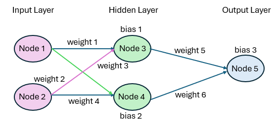
Figure 1 – Simple neural network
This neural network consists of three layers. Each layer consists of one or more nodes. The left-most layer is the Input Layer and consists of two nodes (Node 1 and Node 2). The right-most layer is the Output Layer and consists of one node (Node 5), although the Output Layer may contain more than one node. The middle layer, called the Hidden Layer, contains two nodes (Node 3 and Node 4). A neural network contains one Input Layer, one Output Layer, and any number of Hidden layers.
Basic Concepts
Each node in the Input Layer is connected to all the nodes in the Hidden Layer and each node in the Hidden Layer is connected to all the nodes in the Output Layer. Each such connection has a numerical weight (equivalent to an electric charge in a biological neuron or a slope coefficient in a regression model) and each node in the Hidden or Output layers contains a bias (equivalent to an intercept coefficient in a regression mode).
Signals arriving at the nodes in the Input Layer are translated into signals at each node in the Hidden Layer, which in turn are translated into signals at the nodes in the Output Layer. Thus, signals are transmitted from the Input Layer to the Output Layer. For our purposes, such signals are numeric values.
For example, if x1 is the signal arriving at Node 1 and x2 is the signal arriving at Node 2, then Node 3 in the Hidden Layer is activated by some function of the x1w1 + x2w2 + b1, where w1 and w2 are the weights 1 and 2 (i.e. the weights of the input nodes connected to Node 3), and b1 is the bias at Node 3.
We call this level of activation at Node 3, a3. Similarly, Node 5 in the Output Layer is activated by some function of a3w5 + a4w6 + b3 where a3 is the activation at Node 3 and a4 is the activation at Node 4.
Foreward and Backward Propagation
In general, if the input signal is X = (x1, …, xm) and the resulting output is Y = (y1, …, yn), the neural network can be viewed as calculating a function Y = f(X). Here, we are assuming that there are m nodes in the Input Layer and n nodes in the Output Layer. Our goal is to create a neural network so that Y = f(X) is a function that we are interested in. The process described above for calculating this function is called forward propagation.
Generally, the results of the initial forward propagation, going from left to right through the layers of the network, are not satisfactory. As we shall see, neural networks also use backward propagation, going in the opposite direction, to iteratively update weights and biases until the network is more successful at approximating the function Y = f(X) that we are interested in.
This process is guided by training, in which a training set of (X, Y) values is supplied. At each pass through the training data, the aggregate difference between the Y and f(X) values is measured using a cost function. The cost function plays a role similar to the MSE (minimum squared error) in regression. The objective of backward propagation is to tweak the weights and biases to minimize the cost function. It uses a process called gradient descent.
Notation
We now describe the notation that we will use to make the above description more concrete.
- wh(j, k). Weight of the link between node j of layer h-1 and node k of layer h
- bh(k). Bias for node k of layer h
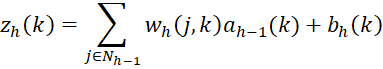
- zh(k). Weighted sum for node k of layer h
- ah(k). Activation for node k of layer h
- σ(z). Activation (link) function
- Nh. The set of nodes in layer h = {1, 2, …, nh}
Formulas
In particular, we use the following formulas where h takes values 2, 3, …, r, where r is the number of the output layer. For a network with one hidden layer, h takes only the values 3 (output layer) and 2 (hidden layer).
![]()
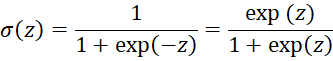
Note that the activation function maps a numeric value between -∞ and +∞ to a value between 0 and 1. This is the same function used in logistic regression.
Cost Function
For a training pair (X, Y) where X = (x1, …, xm) and Y = (y1, …, yn), the cost function that we will use is
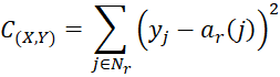
For a set of p training pairs T, we define the cost by
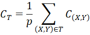
If T is the entire training set under consideration, we denote CT by C.
Links
References
Lubick, K. (2022) Training a neural network in a spreadsheet
https://www.youtube.com/watch?v=fjfZZ6S1ad4
https://www.youtube.com/watch?v=1zwnPt73pow
Nielson, M. (2019) Neural networks and deep learning
http://neuralnetworksanddeeplearning.com/