Multivariate Regression Proofs

Objective

We now provide proofs of properties presented in Multivariate Regression Basic Concepts.

Proofs (part 1)

Property 1: 

B = (X^TX)^-1X^TY

Proof: By univariate regression properties

B = [B₁ B₂ ⋅⋅⋅ B_m]

= [(X^TX)^-1X^TY₁   (X^TX)^-1X^TY₂  ⋅⋅⋅  (X^TX)^-1X^TY_m]

= (X^TX)^-1X^T[Y₁ Y₂ ⋅⋅⋅ Y_m] = (X^TX)^-1X^TY

Property 2: B minimizes the trace

Tr((Y – XB)^T(Y – XB))

Proof: The m × m SSCP matrix S

S = (Y – XB)^T(Y – XB)

has diagonal terms which are non-negative scalars of the form

Now

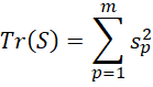
Since the values b_jp minimize each term in the above sum, they also minimize the sum.

Property 3:

E[ε] = 0

Proof: This is a consequence of the fact that E[ε_p] = 0 for all p

Property 4: B is an unbiased estimator of β; i.e. E[B] = β

Proof: By Property 1

B = (X^TX)^-1X^TY

But

Y = Xβ + ε

Thus

B = (X^TX)^-1X^TY = (X^TX)^–1X^T(Xβ+ε)

=(X^TX)^–1X^TXβ + (X^TX)^–1X^Tε

= (X^TX)^–1(X^TX)β + (X^TX)^–1X^Tε

= β + (X^TX)^–1X^Tε

Thus

E[B] = E[β + (X^TX)^–1X^Tε] = E[β] + E[(X^TX)^–1X^Tε]

 = β + (X^TX)^–1X^TE[ε] = β + 0 = β

since E[ε] = 0 by Property 3.

Proofs (part 2)

Property 5:

cov(B_p, B_q) = σ_pq(X^TX)^-1

Proof: Using univariate regression properties

B_p = (X^TX)^-1X^TY_p= (X^TX)^–1X^T(Xβ_p + ε_p)

= (X^TX)^–1X^TXβ_p + (X^TX)^–1X^Tε_p = β_p + (X^TX)^–1X^Tε_p

Thus

B_p = β_p + (X^TX)^–1X^Tε_p

and so

B_p – E[B_p] = β_p + (X^TX)^–1X^Tε_p – β_p = (X^TX)^–1X^Tε_p

Similarly

B_q – E[B_q] = (X^TX)^–1X^Tε_q

Hence

cov(B_p, B_q) = E[((X^TX)^–1X^Tε_p)((X^TX)^–1X^Tε_q)^T]

= E[(X^TX)^–1X^Tε_pε_q^TX(X^TX)^–1] = (X^TX)^–1X^TE[ε_pε_q^T]X(X^TX)^–1

= (X^TX)^–1X^T(σ_pqI)X(X^TX)^–1

The last equality is a result of the fact that E[ε_pε_q^T] = E[(ε_p-E[ε_p])(ε_q-E[ε_q])^T] = cov(ε_p,ε_q) = σ_pqI since E[ε_p] = E[ε_q] = 0. Finally,

cov(B_p, B_q) = (X^TX)^–1X^T(σ_pqI)X(X^TX)^–1

= σ_pq(X^TX)^–1(X^TX)(X^TX)^–1 = σ_pq(X^TX)^–1

Property 6:

E[E_p] = 0

Proof: Here E_p is the pth column of E = [e_ip].

E[E_p] = E[Y_p–XB_p] = E[Y_p] – XE[B_p] = E[Y_p] – Xβ_p

The last equality results from the fact that B_p is an unbiased estimator of β_p.

But

Y_p = Xβ_p + ε_p

and so

E[Y_p] = E[Xβ_p + ε_p] = E[Xβ_p] + E[ε_p] = Xβ_p + 0 = Xβ_p

Putting everything together, we have

E[E_p] = E[Y_p] – Xβ_p = Xβ_p – Xβ_p = 0

Property 7:

cov(Y_p, Y_q) = σ_pq

Proof: 

cov(Y_p, Y_q) = (Y_p – E[Y_p])^T(Y_q – E[Y_q]) = (Y_p –  Xβ_p)^T(Y_q –  Xβ_q)

= ε_p^Tε_q = cov(ε_p, ε_q) = σ_pq

Trace properties

Before we proceed, we recall some properties of the trace of a square matrix. In particular

Property A:

Trace(I_m) = m

Trace(AB) = Trace(BA)

Trace(bA) = bTrace(A)

Trace(A+B) = Trace(A) + Trace(B)

In addition, we prove the following properties.

Property B: For any square matrix A

E[Trace(A)] = Trace(E[A]) 

Proof: For A = [a_ij]

E[Trace(A)] = E[∑a_ii] = ∑ E[a_ii] = Trace(E[A]) 

Property C: For any n × n matrix A and n × 1 matrices Y and Z

E[Y^TAZ] = Trace(A cov(Y,Z)) + E[Y]^TA E[Z]

Proof: First note that AZ is also a n × 1 matrix. Thus, as for any covariance

cov(Y, AZ) = E[Y^TAZ] – E[Y]^TE[AZ]

= E[Y^TAZ] – E[Y]^TA E[Z]

Thus

E[Y^TAZ] = cov(Y, AZ) + E[Y]^TA E[Z]

Also

cov(Y, AZ) = E[(Y–E[Y])(AZ–E[AZ]) = E[(Y–E[Y])A(Z–E[Z])

But cov(Y, AZ) is a scalar, and so cov(Y, AZ) = Trace(cov(Y, AZ)). Using the commutivity property of Trace, we obtain

cov(Y, AZ) = Trace(E[(Y–E[Y])A(Z–E[Z])) = Trace(A E[(Y–E[Y])(Z–E[Z]))

= Trace(A E[(Y–E[Y])(Z–E[Z])) = Trace(A cov(Y, Z))

Putting it all together, we get the desired result

E[Y^TAZ] = cov(Y, AZ) + E[Y]^TA E[Z]

= Trace(A cov(Y,Z)) + E[Y]^TA E[Z]

Hat matrix properties

We now present some properties of the hat matrix

H =  X(X^TX)^–1X^T

Property D: H is symmetric

Proof:

H^T = (X(X^TX)^–1X^T)^T = X((X^TX)^–1)^TX^T = X((X^TX)^T)^-1X^T = X(X^TX)^–1X^T = H

Property E: H is idempotent

Proof:

H² = (X(X^TX)^–1X^T)² = (X(X^TX)^–1X^T)(X(X^TX)^–1X^T)

= X(X^TX)^–1(X^TX)(X^TX)^–1X^T = X(X^TX)^–1X^T = H

Property F: I – H is symmetric and idempotent

Proof: The result follows from Properties D and E since

(I – H)^T = I^T – H^T = I – H

(I – H)² = (I – H)(I – H) = I – 2H + H² = I – 2H + H = I – H

Property G: From Property F, it follows that

(I – H)^T(I – H) = I – H

Property H:

Trace(I – H) = df_Res

Proof: Using Property A

Trace(H) = Trace(X(X^TX)^–1X^T) = Trace(X^TX(X^TX)^–1) = Trace(I) = k+1

Trace(I – H) = Trace(I) – Trace(H) = n – Trace(H) = n – k – 1 = df_Res

Proofs (part 3)

Property 8:

E[E_p^TE_q] = σ_pqdf_Res

Proof: Here df_Res = n – k – 1. First we note that

E_p^TE_q = (Y_p–XB_p)^T(Y_q–XB_q) = (Y_p–HY_p)^T(Y_q–HY_q)

= ((I–H)Y_p)^T((I–H)Y_q) = Y_p^T(I–H)^T(I–H)Y_q = Y_p^T(I–H)Y_q

The last equality follows from Property G. Thus

E_p^TE_q = Y_p^T(I–H)Y_q

By Property C

E[Y_p^T(I–H)Y_q] = Trace((I–H) cov(Y_p, Y_q)) + E[Y_p]^T(I–H)E[Y_q]

By Properties 7 and A,

Trace((I–H) cov(Y_p, Y_q)) = Trace(I–H) ⋅ Trace (cov(Y_p, Y_q))

= df_Res ⋅ Trace (σ_pq) = σ_pq df_Res 

Finally, note that

E[Y_p^T](I–H)E[Y_q] = (Xβ_p)^T(I–X(X^TX)^–1X^T)(Xβ_q)

=(Xβ_p)^T(Xβ_q) – β_p^TX^TX(X^TX)^–1X^TXβ_q = (Xβ_p)^T(Xβ_q) – β_p^TX^TXβ_q = 0

Putting it all together, we have

E[E_p^TE_q]= E[Y_p^T(I–H)Y_q] = Trace((I-H) cov(Y_p, Y_q)) + E[Y_p]^T(I–H)E[Y_q]

= σ_pqdf_Res + 0 = σ_pqdf_Res

Property 9: SSE/df_Res is an unbiased estimate for Σ; i.e. E[SSE] = E[E^TE] = df_ResΣ

Proof: This is a consequence of Property 8.

Property 10:

cov(B_p, E_q) = 0          cov(B, E) = 0

Proof: The proof of the first assertion is similar to that for Property 8. The second assertion follows from the first.

References

Johnson, R. A., Wichern, D. W. (2007) Applied multivariate statistical analysis. 6th Ed. Pearson
https://mathematics.foi.hr/Applied%20Multivariate%20Statistical%20Analysis%20by%20Johnson%20and%20Wichern.pdf

Rencher, A.C., Christensen, W. F. (2012) Methods of multivariate analysis (3^nd Ed). Wiley

Stack Exchange (2011) How to prove that the expression ….
https://math.stackexchange.com/questions/93994/how-to-prove-that-the-expression-ezaz-for-a-random-vector-z-is