Linear Discriminant Analysis

Basic Concepts

In Discriminant Analysis, given a finite number of categories (considered to be populations), we want to determine which category a specific data vector belongs to. More specifically, we assume that we have r populations D₁, …, D_r consisting of k × 1 vectors. Furthermore, we assume that each population has a multivariate normal distribution N(μ_i,Σ_i). The values for μ_i and Σ_i are estimated using training data for which we know which population D_i each X in the training data belongs to.

For each i let f_i(X) be the pdf for N(μ_i,Σ_i), and so we can define f(X|D_i) = f_i(X).

In Linear Discriminant Analysis we assume that Σ1 = Σ₂ = … = Σ_r = Σ, and so each D_i is differentiated by the mean vector μ_i.

Bayesian Approach

We use a Bayesian analysis approach based on the maximum likelihood function. In particular, we assume some prior probability function

We can then define a posterior probability function

For each X we decide which population X belongs to based on maximizing the value of p_i(X). Since for any i the denominator in the expression for p_i(X) is the same (and positive), this is equivalent to maximizing the numerator, i.e. X ∈ D_i* where

and

It now follows that

Since this first term is the same for each i, it can be dropped as it won’t affect the value of i*. This motivates the following definitions.

We now define the linear discriminant function to be

where

and d_i0(X) = d_i0 and d_ij(X) = d_ij.

We also define the linear score to be s_i(X) = d_i(X) + LN(π_i). As we demonstrated above, i* is the i with the maximum linear score.

Using the training data, we estimate the value of μ_i by the mean of the X_i = the average of all the training data in D_i. Similarly, we estimate the value of Σ by the pooled sample covariance matrix S. More precisely, let S_i be the covariance matrix for D_i, then the pooled covariance matrix is

where n_i = the number of elements in D_i. Thus, we estimate the various linear scores using

We can assign the prior probability functions π_i(X) based on our best available prior information, as long as π_i(X) = 1 and π_i(X) > 0 for all i.

In particular, if we assume that all populations are equally likely then we can choose

If we assume that the probability is weighted by the population size then

The posterior probability that  is given by the formula

Examples

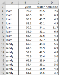
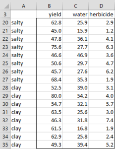
Example 1: Perform discriminant analysis on the data in Example 1 of MANOVA Basic Concepts. This data is repeated in Figure 1 (in two columns for easier readability). Also determine in which category to put the vector X with yield 60, water 25 and herbicide 6.

Figure 1 – Training Data for Example 1

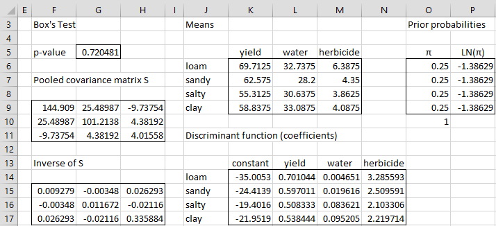
The analysis begins as shown in Figure 2. First, we perform Box’s M test using the Real Statistics formula =BOXTEST(A4:D35). Since p-value = .72 (cell G5), the equal covariance matrix assumption for linear discriminant analysis is satisfied. The other assumptions can be tested as shown in MANOVA Assumptions.

We next calculate the pooled covariance matrix (range F9:H11) using the Real Statistics array formula =COVPooled(A4:D35). The inverse of this matrix is shown in range F15:H17, as calculated by the Excel array formula =MINVERSE(F9:H11).

The mean vector for the loam population is displayed in range K6:M6, with the mean vectors for the other three populations shown just below it. These values are calculated by putting the formula

=AVERAGEIF($A$4:$A$35,$J6,B$4:B$35)

in cell K6, highlighting the range K6:M9 and pressing Ctrl-R and Ctrl-D.

Figure 2 – Discriminant Analysis

We will assume that a prior all four categories are equally likely and so we set the prior probabilities to 25% as shown in range O6:O9. The LN for each of these values is shown in range P6:P9.

Finally, we calculate the coefficients of the discriminant analysis in range K14:N17. Here, K14 contains the value of d₁₀, as calculated by the array formula

=-0.5*MMULT(K6:M6,MMULT($F$15:$H$17,TRANSPOSE(K6:M6)))

The remaining d_1j coefficients (for loam) are calculated by inserting the following array formula in range L14:N14

=MMULT(K6:M6,$F$15:$H$17)

Highlighting the range K14:N17 and pressing Ctrl-D, we fill in the d_ij coefficients for the other three categories.

We now determine in which category to put the vector X with yield 60, water 25 and herbicide 6 (see Figure 3).

Figure 3 – Determining the best category

First, we determine the score for each category i using the formula

For example, the score for loam is 25.50092, as calculated using the formula

=$K$14+SUMPRODUCT(S38:U38,$L$14:$N$14)+$P$6

The scores for the other three categories are calculated in a similar manner using the discriminant coefficients and prior probability. We see that the score for sandy is the highest and so we use that as the category for X (cell Z38). Note that this category can be determined by the following formula:

=INDEX($V$3:$Y$3,,MATCH(MAX(V38:Y38),V38:Y38,0))

The posterior probability that X is in the loam population is shown in cell V39, as calculated by the formula

=EXP(V$38)/SUMPRODUCT(EXP($V$38:$Y$38))

which is 35.2%. There is a 37.6% probability that it will be classified as sandy (cell W39), and so we are only 37.6% confident that X is in the sandy population (i.e. a 62.4% error rate). Whether this is a sufficiently high level of confidence depends on the cost of being wrong and the reward for being right. If we are predicting which women have cancer based on a mammogram, we would clearly require a much higher level of confidence.

Reference

Penn State (2017) Linear discriminant analysis. STAT 505 Applied Multivariate Statistical Analysis
https://online.stat.psu.edu/stat505/lesson/10/10.3