Traditional Approaches for Handling Missing Data

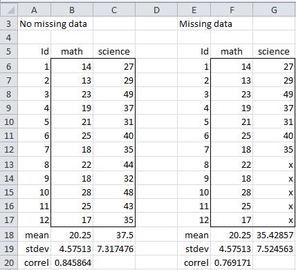
We now turn our attention to some of the methods used for handling missing data. In particular, we will start by looking at the data shown in Figure 1.

Figure 1 – Missing Data

Here we see that 5 of the 12 data elements are missing. We show the full data set without any missing data as well. Keep in mind that in practice we will almost never have the luxury of knowing what the missing data values are really supposed to be.

Listwise deletion

Probably the most commonly used approach when the data range has some missing data elements is to eliminate any rows with missing data, i.e. to eliminate the ith row of X if one or more x_ij is missing for j = 1, …, k. This is called listwise deletion or complete case analysis (CCA).

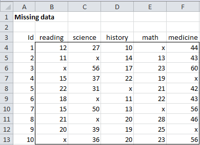
As described in Dealing with Missing Data, this approach can be reasonable when there is only a small amount of missing data. But even a small amount of missing data can result in a large percentage of the sample being deleted. For example, even though only 20% of the data in Figure 2 is missing, no data is left after listwise deletion.

Figure 2 – Each case has some missing data

Even in less extreme cases, unless the original data set was quite large the reduced sample size can dramatically reduce the power of whatever test is performed.

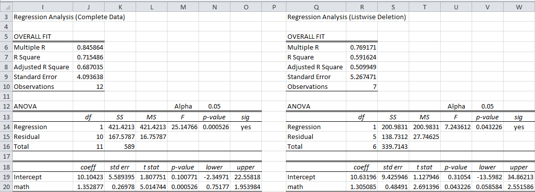
Referring to Figure 1, if we compare the regression model of the complete data (all 12 rows in range B6:C17) with that of the data using listwise deletion (7 rows in the range F6:G12) we get the results shown in Figure 3.

Figure 3 – Comparison of Regression Models

As we can see, the regression model for the complete data looks to be a better fit than for the incomplete data (Adjusted R of .687 vs. .509). Consequently, it appears that something is lost by eliminating 5 of 12 rows (41.7% of the data) even though only 5 of 24 data elements (20.8%) are missing.

Single imputation using the mean

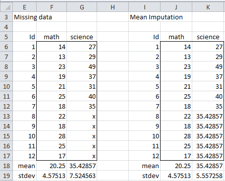
As described in Dealing with Missing Data, we can impute the value of any missing data based on the values of the non-missing data. A simple approach is to fill in the values of the missing science values in Figure 1 with the value of the mean of the non-missing data, namely 35.4287 (cell G18). This is shown in Figure 4.

Figure 4 – Mean Imputation

The result is that the standard deviation of the science variable has decreased from 7.525 to 5.557. This is not surprising since the deviations for these last five data elements are 0. That we get biased values for the standard deviation is clearly not very desirable.

Single imputation using regression

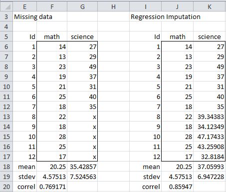
Another approach for filling in the missing data is to use the forecasted values of the missing data based on a regression model derived from the non-missing data. Figure 5 displays the results of this approach for the data in Figure 1.

Figure 5 – Regression imputation

This time we impute the values of the five missing cells by inserting the array formula =FORECAST(J13:J17,G6:G12,F6:F12) in the range K13:K17. Since this results in a perfect linear correlation between the math and science values for the last five data elements, it is not surprising that the correlation coefficient between math and science rises from .769 (cell F20) to .859 (cell J20). The standard deviation also falls. Regression imputation creates biased values for the correlation coefficient and standard deviation (although if the data is MAR or MCAR the mean is not biased). Once again this is not desirable.

Note that the estimate for the correlation coefficient produced by this approach is quite close to that observed for the complete data (cell B20 of Figure 1) since the correlation there is already quite high. The standard deviation is again lower than that for the complete model (cell C19 of Figure 1).

Single imputation using stochastic regression

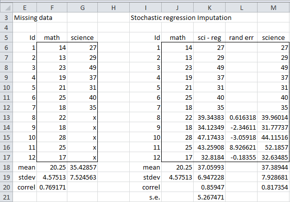
We can improve the situation by adding a random component to the imputed regression values. This will artificially increase the variability. The approach used is to simply add a randomly generated value following the normal distribution N(0, s.e.) where s.e. is the standard error of the regression model on the non-missing data. Figure 6 displays the results of this approach for the data in Figure 1.

Figure 6 – Stochastic regression imputation 

The value of the standard error for the regression is s.e. = 5.267, as shown in cell R9 of Figure 3 (and duplicated in cell K21 of Figure 6). Thus we need to add the random error value calculated by the formula

=NORM.INV(RAND(),0,K$21)

to each of the imputed values shown in Figure 5 (and duplicated in Figure 6). These values (shown in column L of Figure 6) when added to the regression imputed values yield the stochastic regression values shown in column M of Figure 6.

This time the standard deviation is increased and the correlation is decreased, as we had hoped. The actual adjustment, however, depends on the random numbers generated to create the random errors. These can be quite volatile.

Examples Workbook

Click here to download the Excel workbook with the examples described on this webpage.

References

Baraldi, A. N. and Enders, C. K. (2010) An introduction to modern missing data analyses, Journal of School Psychology 48, 5–37.
https://pubmed.ncbi.nlm.nih.gov/20006986/

Eekhout, I. (2019) Single imputation methods. Don’t miss out.
https://www.missingdata.nl/missing-data/missing-data-methods/imputation-methods/

Hain, H. (2021) Stochastic regression imputation
This document is no longer available online.