Multiple Regression using FIML

In the other web pages on the FIML topic, we have used the FIML procedure to determine the most likely fit for the population covariance matrix and mean vector based on the sample data even with missing data. We now use the estimate for the population covariance matrix to derive a multiple regression model for the data.

Example

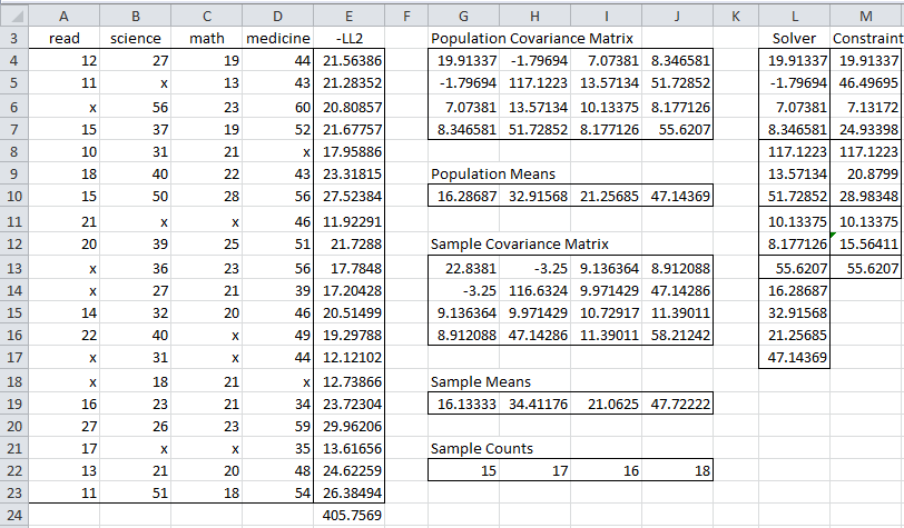
An example of the results of this procedure is shown in Figure 3 of FIML using Solver, which is replicated below in Figure 1.

Figure 1 – Output from FIML procedure using Solver

Until now all four variables in the example have been treated in the same way. Now we will assume that the medicine variable is the dependent variable and the other three variables are independent variables.

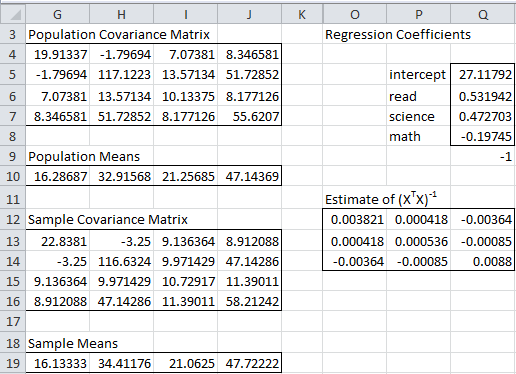
We begin by calculating the regression coefficients, as shown in range Q5:Q8 of Figure 2.

Figure 2 – Regression coefficients and their standard errors

The left side of Figure 2 just contains a copy of columns G through J from Figure 1. In particular, the population covariance matrix is the result of using Solver, as described above.

Regression coefficients

By Property 1 of Multiple Regression Least Squares, we can obtain the non-intercept regression coefficients (range Q6:Q8) via the formula

=MMULT(MINVERSE(G4:I6),J4:J6)

The intercept coefficient (cell Q5) can be calculated by the array formula

=-MMULT(G10:J10,Q6:Q9)

Standard errors of the coefficients

To calculate the standard errors of these coefficients, we first need to estimate (X^TX)^-1 in range O12:Q14. If we ignore the intercept, then we have two approaches, the first based on the sample covariance matrix

=MINVERSE(G13:I15)/(COUNTA(A4:A23)-1)

and the second based on the population covariance matrix

=MINVERSE(G4:I6)/(COUNTA(A4:A23))

We elect to use the first of these approaches, but it is easy to modify the result to use the second approach. Note that when there is no missing data, the two approaches are equivalent. In order to obtain the covariance matrix for the regression coefficients, we need to multiply (X^TX)^-1 by MS_Res. We will show how to calculate MS_Res shortly.

Regression model

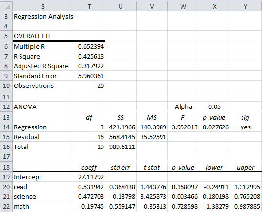
Figure 3 contains the multiple regression model.

Figure 3 – Multiple regression using FIML

Most of the fields are calculated as in the multiple regression model described in Figure 13 of Multiple Regression Analysis.

R-square and SSTot

We first show how to calculate R². To do this we note that

and so we can use the formula

=SUMPRODUCT(J13:J15,Q6:Q8)/J16

to calculate R² (cell T7). We next estimate the value of SS_T by the formula (referring to Figure 1):

=DEVSQ(D4:D23)

Since two values for the read variable are missing, this formula underestimates the value of SS_T. Since there are 18 non-missing values for the read variable out of the 20 rows in the sample, we could multiply this estimate for SS_T by 20/18; i.e. in general we estimate  by

=DEVSQ(D4:D23) * COUNTA(D4:D23) / COUNT(D4:D23)

Alternatively, we could simply eliminate all the rows where the dependent variable is missing a value before we start the FIML procedure.

SSReg and SSRes

We next estimate SS_Reg and SS_Res using the formulas

Thus SS_Reg (cell U14) can be calculated by the formula

=U16*T7

and SS_Res (cell U15) can be calculated by the formula

=U16-U14

Other elements

All the other entries in the ANOVA table are calculated in the usual way. In particular, MS_Res (cell V15) is calculated by the formula

=U15/T15

and so the standard error (cell T9) is calculated by the formula

=SQRT(V15)

All the other entries in the Overall Fit table are calculated in the usual way. We now turn our attention to the coefficients table. The coefficients (range T19:T22) can be calculated by (referring to Figure 2):

=Q5:Q8

The standard errors of the coefficients (range U20:U22) are calculated by (referring to Figure 2):

=T9*SQRT(DIAG(O12:Q14))

All the other entries in the coefficients table are calculated in the usual way, thus completing the description of Figure 3.

Note that we used the value 20, via the formula =COUNTA(A4:A23), for the number of observations (cell T10). Since there are missing data elements, there are grounds for replacing this amount with the average of the number of non-missing elements in the sample for each of the four variables. Referring to Figure 1, this can be calculated by the formula

=AVERAGE(G22:J22)

resulting in a value of 16.5. If we use this value then the df values would also get modified.

Examples Workbook

Click here to download the Excel workbook with the examples described on this webpage.

References

Enders, C. K. (2001) The performance of the full information maximum likelihood estimator in multiple regression models with missing data. Educational and Psychological Measurement, Vol. 61 No. 5.
https://asu.elsevierpure.com/en/publications/the-performance-of-the-full-information-maximum-likelihood-estima

Allison, P. D. (2012) Handling missing data by maximum likelihood
https://statisticalhorizons.com/wp-content/uploads/MissingDataByML.pdf