Initialization of FIML

Basic Setup

On this webpage, we show how to initiate the FIML procedure in Excel. In particular, we use the data in range A3:E23 of Figure 1 to illustrate how this is done using Excel’s Solver.

Figure 1 – Description of Missing Data

Before we carry out the FIML procedure we would like to look at the missing data summaries displayed on the right side of Figure 1. In particular, we use the following worksheet function.

Worksheet Function

Real Statistics Function: The Real Statistics Resource Pack furnishes the following array function where R1 is a range such as B3:E23 in Figure 1 if head = TRUE or B4:E23 in Figure 1 if head = FALSE (default).

MissingPairwise(R1, head) – generates a summary of the percentage of non-missing data for each pair of variables in R1. If head = TRUE then the output also includes row and column headings.

The pairwise non-missing data report in range G4:K8 is generated by =MissingPairwise(B3:E23,TRUE). The sample covariance matrix in range H13:K17 is generated by the formula =COV(B4:E23,FALSE) as described in Multiple Regression Least Squares. The descriptive statistics report in range G20:K25 is generated by the formula =DescStats(B3:E23,TRUE,TRUE) as described in Multiple Imputation using FCS.

Minimum -2LL Value

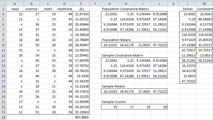
To find the minimum value of -2LL for the data in Figure 1, we need to add a column that calculates the value of LL_i for each row i in Figure 1. This is shown in Figure 2.

Figure 2 – Initialization of the FIML procedure

The added column appears in column E of Figure 2. The elements in this column are based on the values of the population covariance matrix (range G4:J7) and population mean vector (G10:J10). These are both initiated to be the corresponding sample values.

The sample covariance matrix (range G13:J16) is calculated by the array formula =COV(A4:A23,FALSE). The sample mean for the read variable (cell G19) is calculated by the formula =AVERAGE(A4:A23), and so by highlighting the range G19:J19) and pressing Ctrl-R we calculate all the values in the sample mean vector.

Initial -2LL Value

We now show how to calculate the initial value of -2LL₁ (cell E4). Since the first row of data contains no missing data elements, k₁ = k, μ₁ = μ, and Σ₁ = Σ, and so

which can be calculated by the Excel array formula

=MMULT(A4:D4-G10:J10,MMULT(MINVERSE(G4:J7),TRANSPOSE(A4:D4-G10:J10))) + COUNT(A4:D4)*LN(2*PI()) + LN(MDETERM(G4:J7))

The value of this formula is 21.87163.

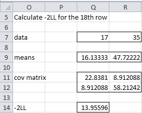
To calculate the initial value of -2LL₁₈ (cell E21), we need to filter out the two missing values as well as filter the mean vector and covariance matrix as described in FIML Basic Concepts.

Figure 3 – Reduced ranges for rows with missing data 

The filtered data, mean vector, and covariance matrix are shown in Figure 3. Thus the initial value of -2LL₁₈ can be calculated by the array formula

=MMULT(Q7:R7-Q9:R9,MMULT(MINVERSE(Q11:R12),TRANSPOSE(Q7:R7-Q9:R9))) + COUNT(Q7:R7)*LN(2*PI()) + LN(MDETERM(Q11:R12))

which has the value 13.95596.

Fortunately, we don’t have to make these calculations each time but instead can use the following function.

Worksheet Function for -2LL

Real Statistics Function: The Real Statistics Resource Pack furnishes the following array function where R1 is a 1 × k row vector, R2 is a k × k covariance matrix and R3 is a 1 × k mean vector.

LLReg(R1, R2, R3) – the value of -2LL_i for the row represented by R1, possibly containing missing data.

Thus

LLReg(A4:D4,G4:J7,G10:J10) = 21.87163

LLReg(A21:D21,G4:J7,G10:J10) = 13.95596

The value -2LL (cell E24 of Figure 2) is therefore the sum of the values of -2LL_i for all the rows, and so can be calculated by the formula =SUM(E4:E23).

Examples Workbook

Click here to download the Excel workbook with the examples described on this webpage.

References

Enders, C. K. (2001) The performance of the full information maximum likelihood estimator in multiple regression models with missing data. Educational and Psychological Measurement, Vol. 61 No. 5.
https://asu.elsevierpure.com/en/publications/the-performance-of-the-full-information-maximum-likelihood-estima

Allison, P. D. (2012) Handling missing data by maximum likelihood
https://statisticalhorizons.com/wp-content/uploads/MissingDataByML.pdf