Correlation Testing for more than two samples

Omnibus Test

Suppose you have k sample pairs with sizes n₁, n₂, …, n_k and correlations r₁, r₂, …, r_k, then you can test the null hypothesis H0: ρ₁ = ρ₂ = ⋅⋅⋅ = ρ_k using the test statistic

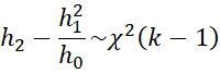
where

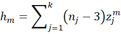
If the null hypothesis is not rejected, then this is evidence that you can combine all the samples and estimate the population correlation by the combined sample correlation coefficient. In particular, you can estimate the population correlation by using the inverse Fisher transformation on the weighted z, namely

z_w = h₁ / h₀

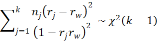
Note that the Fisher transformation (see Correlation Test using the Fisher Transformation) introduces some bias, which may impact the results for the test with more than two samples. A less biased test is as follows:

Null hypothesis not rejected

If the null hypothesis is not rejected you can also test

H0: ρ = 0 using the test statistic

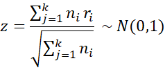
As usual, the null hypothesis is rejected if |z| ≥ z_α/2 (critical value for standard normal distribution at α/2).

For the one-sided test, the null hypothesis H0: ρ ≤ 0 is rejected if z ≥ z_α (critical value for standard normal distribution at α).

The null hypothesis H0: ρ >= 0 is rejected if z ≤ –z_α

If the null hypothesis is not rejected you can also test

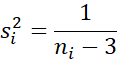
H0: ρ = ρ₀ using the test statistic

where z₀ = the Fisher transformation of ρ₀.

Example 1

Determine whether ρ₁ = ρ₂ = ρ₃ based on the three samples characteristics of three samples provided in range A1:D3 of Figure 1.

Using the first of the tests described above, we see that we can’t reject the null hypothesis (p-value = .867). Note that range G4:G7 displays the formulas used in B4:B7.

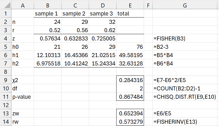
Figure 1 – Chi-square test 1

We get a similar result using the second test, as shown in Figure 2.

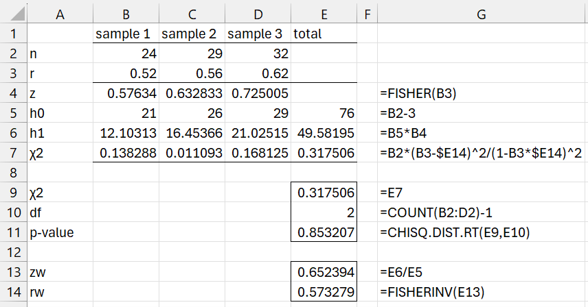
Figure 2 – Chi-square test 2

That we haven’t rejected the null hypothesis is consistent with the three samples coming from the same population. The estimate for the correlation rho from this population is .5733 as shown in cell E14.

We now test the null hypothesis that ρ = 0 as shown in Figure 3.

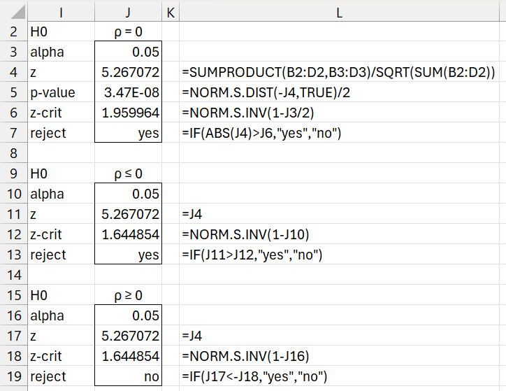
Figure 3 – ρ = 0 test

We see from Figure 3 that the null hypothesis is rejected. The figure also displays the test for the two one-tailed tests. Not surprisingly, the null hypothesis ρ ≥ 0 is not rejected.

In Figure 4, we instead test the null hypothesis ρ = .7. This null hypothesis is not rejected.

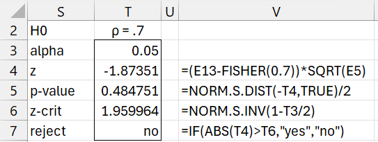
Figure 4 – ρ = .7 test

Null hypothesis rejected

If the null hypothesis is rejected you can perform Tukey HSD post-hoc tests.

To compare the jth and mth samples, you use the test statistic

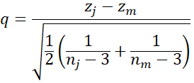
We use the  Studentized Range q Table with critical value q_k,∞,α

We can also use Dunnett’s test where z_m is Fisher(r_m) for the control. The test statistic is the same as q except that the ½ under the square root is removed.

Finally, we can test contrasts using the test statistic

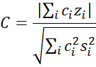
where

Actually, we will use the following test statistic

Example 2

Determine whether ρ₁ = ρ₂ = ρ₃ based on the three samples characteristics of three samples provided in range A1:D3 of Figure 5.

Using the first of the tests described above, we reject the null hypothesis (p-value = .008754). The results for the other test are similar (p-value = .008362).

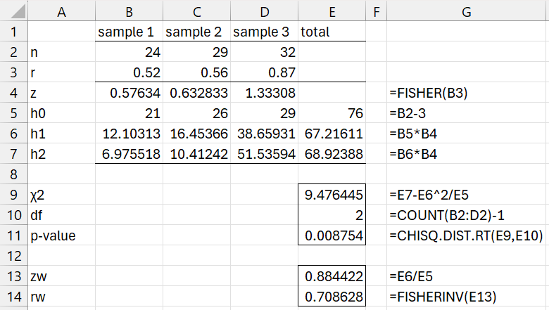
Figure 5 – Reject the null hypothesis

We now use the Tukey HSD test to determine which pairwise comparisons are significant, as shown in Figure 6. Column N displays the formulas in column L.

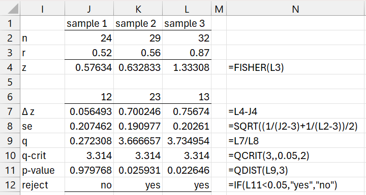
Figure 6 – Tukey HSD follow-up testing

We see that the comparisons 23 and 13 are significant.

If sample 1 represents the control, then we could use Dunnett’s test to see which comparisons 12 and/or 13 are significant. This analysis is displayed in Figure 7.

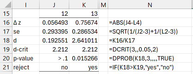
Figure 7 – Dunnett’s follow-up testing

This test shows that the comparison between the control and sample 3 is significant while the comparison between the control and sample 2 is not.

Finally, we show how to conduct contrast analysis comparing the mean of samples 1 and 2 with sample 3, as shown in Figure 8.

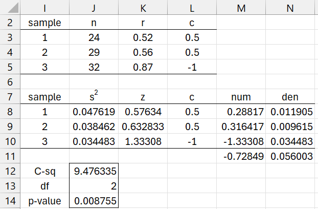
Figure 8 – Contrast analysis

We see that the contrast is significant (p-value = .008755).

Figure 9 displays representative formulas from Figure 8.

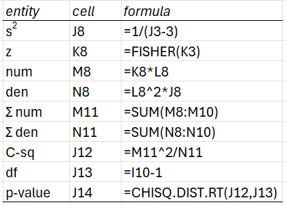
Figure 9 – Representative formulas

Worksheet Functions

Click here for information about Excel worksheet functions supplied by the Real Statistics Resource Pack.

Examples Workbook

Click here to download the Excel workbook with the examples described on this webpage.

Reference

Zar, J. H. (2010) Biostatistical analysis 5^th Ed. Pearson
https://www.scribd.com/document/481055909/