Objective
In Bayesian Two-Sided Testing we describe how to perform the equivalent of a two-tailed t-test using a Bayesian framework. On this webpage, we provide examples in Excel.
One-sample examples
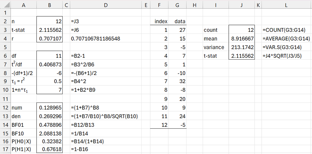
Example 1: Test the null and alternative hypotheses for the revised data for Example 2 of Bayesian One-sided Hypothesis Testing (repeated in range G3:G14 of Figure 1 below) using a scaled information prior with r = .707.
H0: μ = 0
H1: μ ≠ 0
The left side of Figure 1 shows the calculation of BF01, BF10, P(H0|X), and P(H1|X) based on the values n, t, and r shown in range B2:B4. If you supply these values, then you can perform the analysis.
The right side of Figure 1 shows how to calculate n and t based on the data in column G.
Figure 1 – One-sample test using scaled information prior
We see that the alternative hypothesis is favored with BF10 = 2.09, which is barely worth mentioning. The probability that μ = 0 is about 1/3 and the probability that μ ≠ 0 is about 2/3.
Sensitivity Analysis
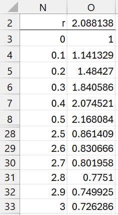
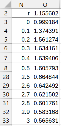
It is useful to see how sensitive these results are to the original choice of the scale parameter r. We can create a chart to evaluate this by using Excel’s Data Table capability. We enter values for r between 0 and 3 as shown in range N3:N33 of Figure 2 (the middle values are not displayed).
Figure 2 – Data Table
You then insert the formula =B15 in cell O2 (pointing to the BF10 cell in Figure 1), highlight the range N2:O33, and select Data > Forecast|What-If Analysis > DataTable… from the ribbon. You then insert B4 (which points to the r cell in Figure 1) in the Column input cell field of the dialog box that appears. Excel now fills in column O with the BF10 values that correspond to each of the r values.
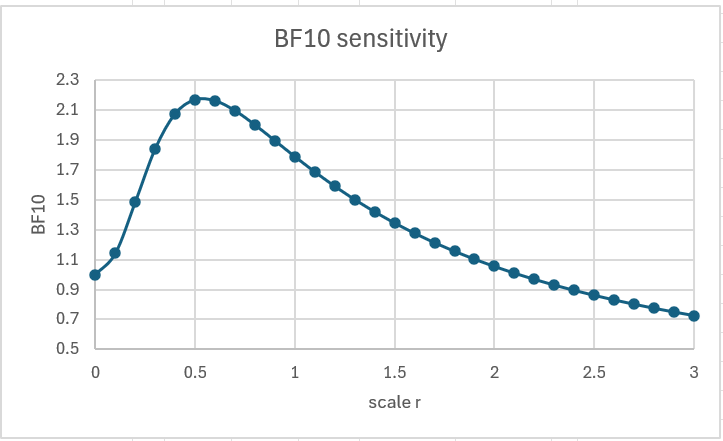
Next, we highlight range N3:O33 and select Input > Charts|Scatter > Scatter with Smooth Lines and Markers from the ribbon. This results in a chart similar to that shown in Figure 3.
Figure 3 – Sensitivity Analysis
We see that the curve is fairly flat around r = .707, obtaining a peak at about r = .538 with BF10 = 2.175. We also see that if we make r too large, then the test favors the null even though it is more likely that the alternative hypothesis holds.
Furthermore, we see that if we had selected r = 1, then BF10 = 1.79, which still favors the alternative hypothesis.
JZS Prior
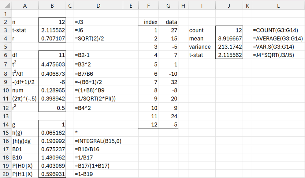
Example 2: Repeat Example 1 using the JZS prior.
The results are shown in Figure 4.
Figure 4 – One-sample test using JZS prior
The formula in cell B15 is
=1/SQRT(1+B$2*B$12*B14)*(1+B$7/(B$6*(1+B$2*B$12*B14)))^B$9*B$11*B14^(-3/2)*EXP(-1/(2*B14))
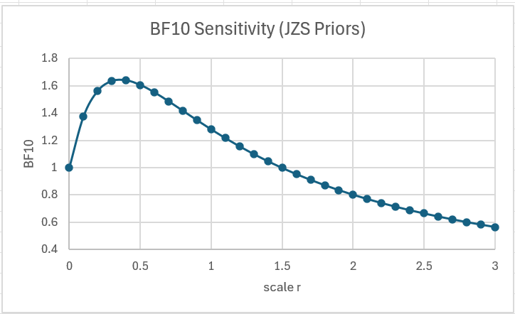
Once again, we can use Excel’s Data Table capability and a scatter chart to obtain the results in Figures 5 and 6.
Figure 5 – Data Table (JZS Priors)
Figure 6 – Sensitivity Analysis (JZS Priors)
Paired-sample examples
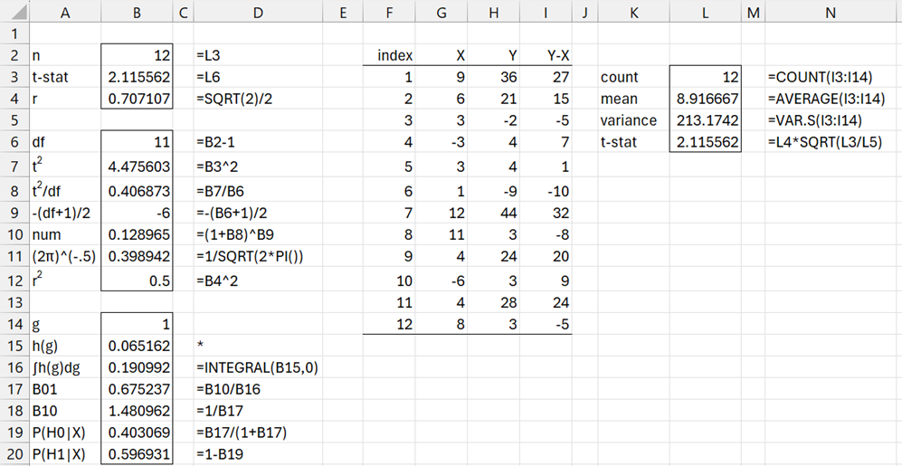
Example 3: Test the null and alternative hypotheses for the paired data shown in range G2:H14 of Figure 7 using a JZS prior with r = .707.
As usual, this is equivalent to a one-sample test on the difference between the paired values. The analysis is shown in Figure 7 and is equivalent to the analysis shown in Figure 4.
Figure 7 – Paired sample test using JZS prior
Two independent samples examples
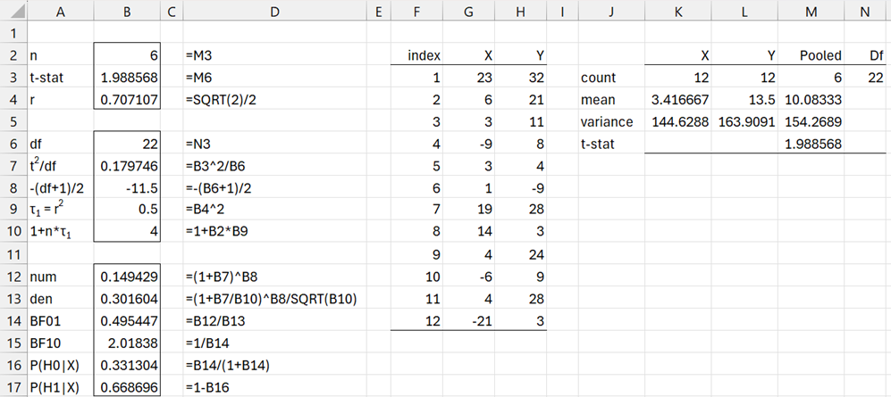
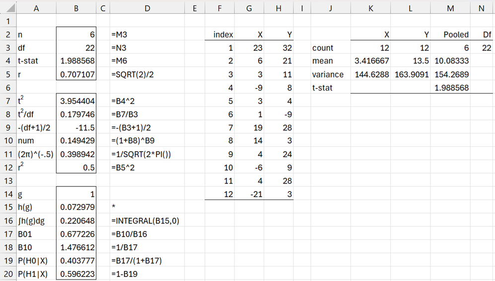
Example 4: Test the null and alternative hypotheses for two independent samples using a scaled information prior with r = .707 based on the data in range G2:H14 of Figure 8.
H0: μ1 = μ2 (equivalent to δ = 0)
H1: μ1 ≠ μ2 (equivalent to δ ≠ 0)
where δ = (μ2 – μ1)/σ.
The analysis is shown in Figure 8. Cell M3 contains the formula =K3*L3/(K3+L3) and cell N3 contains the formula =K3+L3-2. Cell M5 contains =((K3-1)*K5+(L3-1)*L5)/N3 and cell M6 contains =M4*SQRT(M3/M5).
Figure 8 – Two-sample test using scaled information prior
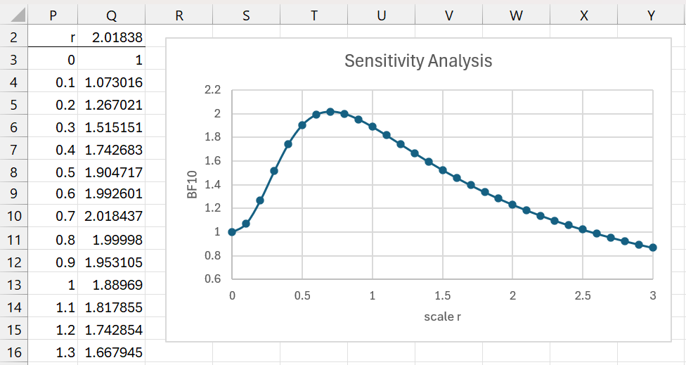
Note that despite the wide difference between the means for X and Y, the BF10 = 2.018 is barely worth mentioning. In the frequentist approach, p-value = .06, which is not significant.
The sensitivity analysis is shown in Figure 9.
Figure 9 – Sensitivity Analysis
JZS Prior
Example 5: Repeat Example 4 using the JZS prior.
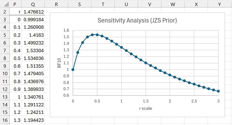
The results are shown in Figures 10 and 11.
Figure 10 – Two-sample test using JZS prior
Figure 11 – Sensitivity Analysis (JZS Prior)
Examples Workbook
Click here to download the Excel workbook with the examples described on this webpage.
References
Stack Exchange (2022) Understanding the Jeffreys-Zellner-Siow (JZS) prior in Bayesian t-tests
https://stats.stackexchange.com/questions/570605/understanding-the-jeffreys-zellner-siow-jzs-prior-in-bayesian-t-tests
Rouder, J. N. et al. (2009) Bayesian t tests for accepting and rejecting the null hypothesis
https://www.researchgate.net/publication/24207221_Bayesian_t_test_for_accepting_and_rejecting_the_null_hypothesis
Gonen, M., Lu, Y., Johnson, W. O., Westfall, P. H. (2005) The Bayesian two-sample t-test
https://scispace.com/pdf/the-bayesian-two-sample-t-test-2cf8tnzpmi.pdf
Du, H., Edwards, M. C., Zhang, Z. (2019) Bayes factor in one-sample tests of means with a sensitivity analysis: a discussion of separate prior distributions
https://link.springer.com/content/pdf/10.3758/s13428-019-01262-w.pdf
Faukenberry, T. (2023) Bayesian t-tests
https://www.youtube.com/watch?v=D4RJk3SmhUY
